Rectangular Waveguide (rectangularWaveguide.sdf)
Keywords:
- Field Boundary Condition, rectangularWaveguide, Rectangular Waveguide
Problem description
This example illustrates how to create a rectangular waveguide using the Rectangular Waveguide Field Boundary Condition and Constructive Solid Geometry.
Three waveguides are demonstrated in this example .
Opening the Simulation
The Rectangular Waveguide example is accessed from within VSimComposer by the following actions:
Select the New → From Example… menu item in the File menu.
In the resulting Examples window expand the VSim for Vacuum Eletronics option.
Expand the Cavities and Waveguides option.
Select Rectangular Waveguide and press the Choose button.
In the resulting dialog, create a New Folder if desired, and press the Save button to create a copy of this example.
The Setup Window is shown in Fig. 368.
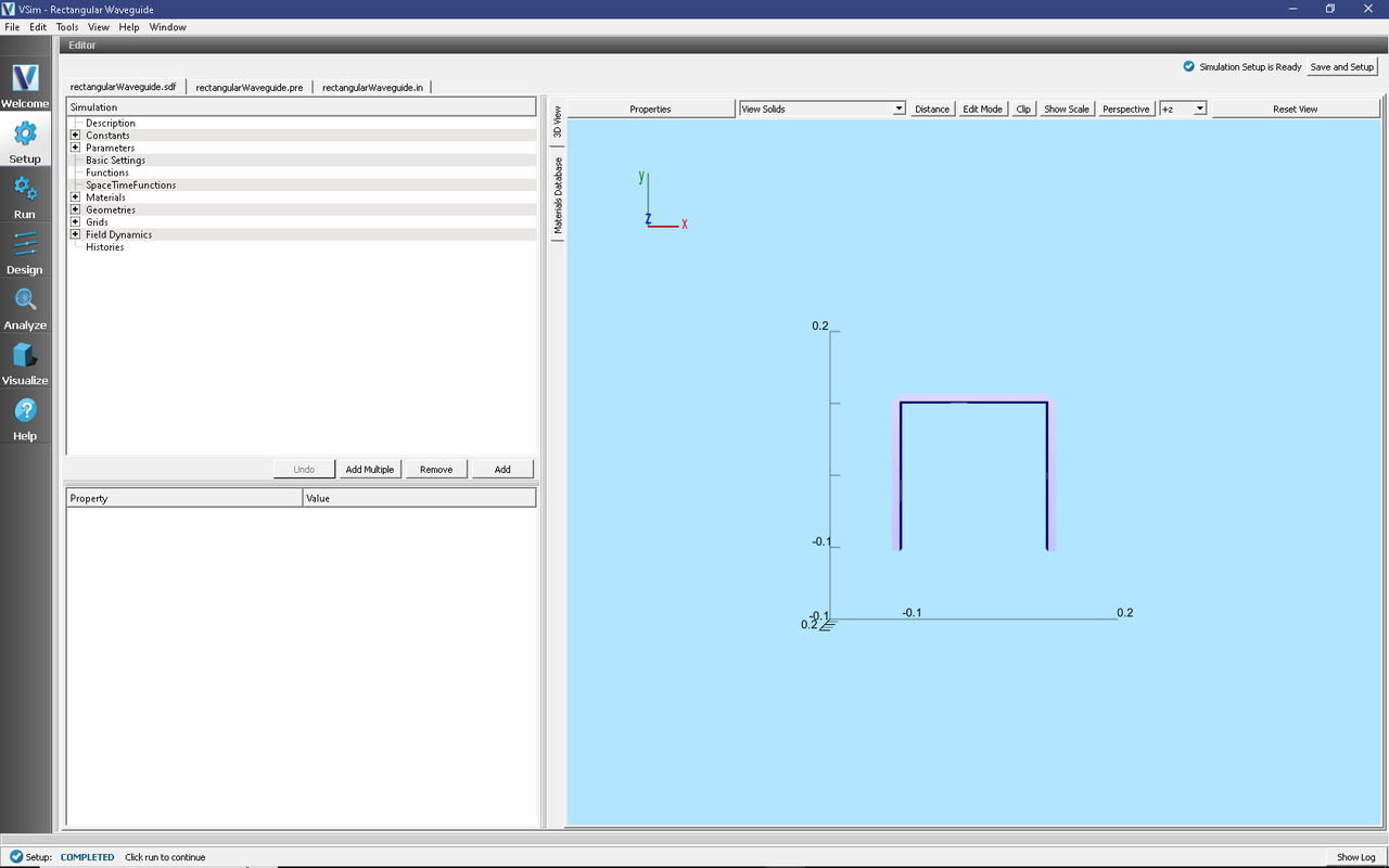
Fig. 368 Setup Window for the Rectangular Waveguide example.
Simulation Properties
This simulation demonstrates how to create a rectangular waveguide. There are three rectangular waveguides in this simulation. Each has been constructed by creating a physical waveguide on the simulation boundary, and defining the wave that is carried into the simulation. First a metal plate from a box primitive has been placed on the simulation boundary. It is important that this plate extends from at least one cell outside of the simulation boundary to at least one cell inside of the simulation. Next a box primitive corresponding to the size and orientation of the actual waveguide has been created. This is then subtracted from the previously created metal plate. It is important to note here that the polarization parameter will always be parallel to the width. The wave carried in this waveguide is then created by adding a FieldBoundaryCondtion of Rectangular Waveguide. The waveguide surface must be specified to match the intended simulation boundary and on the right location to match the physically constructed waveguide.
Several standard waveguide sizes are available, or User-Defined may be selected to specify a custom size. If no “Turn On Time” is specified, it will be set to a time of 2.5 periods of the carried signal, and a warning will be provided after running the simulation.
Running the Simulation
Once finished examining the problem setup, continue as follows:
Proceed to the Run Window by pressing the Run button in the left column of buttons.
Use the default values for the stepping.
Choose parallel computing options if desired
To run the file, click on the Run button in the upper left corner of the right pane. You will see the output of the run in the right pane. The run has completed when you see the output, “Engine completed successfully.” This is shown in the window below.
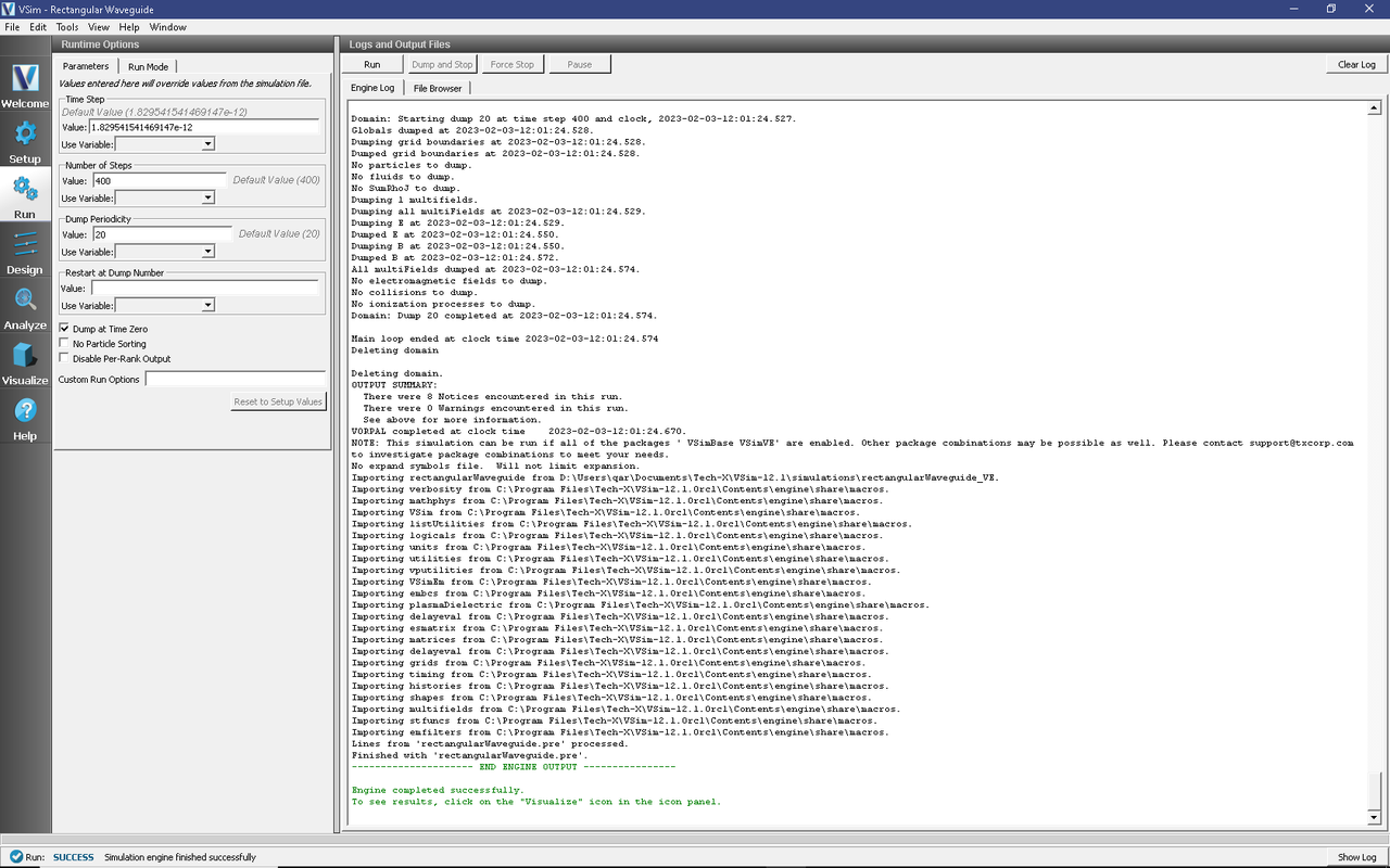
Fig. 369 The Run Window at the end of execution.
Visualizing the Results
After a successful run, go to the Visualize Window by pressing Visualize in the left column.
Expand Scalar Data, E, and select \(E_{y}\). To slice inside the field, check the Clip Plot box. Now step through time using the Dump slider on the bottom of the right pane. This is shown below.
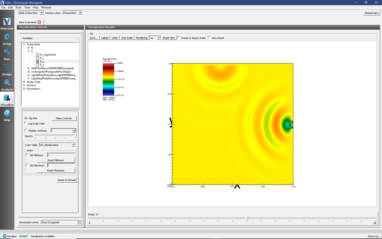
Fig. 370 The \(E_{y}\) field propagating out of the two waveguides centered on the z axis.
The effects of the third waveguide can be viewed by adjusting the “Origin of Normal Vector” parameter under the Plane Controls button.
Further Experiments
Waveguides can be added or subtracted to this simulation.