A15 Crab Cavity (crabCavityT.pre)

Keywords:

electromagnetic cavities, accelerators, mode frequencies

Problem Description

The Crab Cavity simulation illustrates how to extract the modes and frequencies of an accelerator cavity in a given frequency range. The range of interest here is 3.9 to 4.1 GHz. The simulation is performed by exciting the cavity with a broadly filtered pulse that excites modes in a given range. The excitation occurs through a temporally and spatially specified current source that excites the frequencies of interest. The simulation features a variable sampling frequency, allowing the cavity to first be rung up without generating excessive memory dumps. After the simulation has been rung up, sampling frequency increases, and when combined with post-processing find the modes and frequencies. The algorithm is detailed in [1].

This simulation can be performed with a VSimEM, VSimVE or VSimPD license.

Opening the Simulation

The Crab Cavity example is accessed from within VSimComposer by the following actions:

• Select the New → From Example… menu item in the File menu.

• In the resulting Examples window expand the VSim for Microwave Devices option.

• Expand the Cavities and Waveguides (text-based setup) option.

• Select “A15 Crab Cavity (text-based setup)” and press the Choose button.

• In the resulting dialog, create a New Folder if desired, and press the Save button to create a copy of this example.

The basic variables of this problem should now be alterable via the text boxes in the left pane of the Setup Window, as shown in Fig. 385.

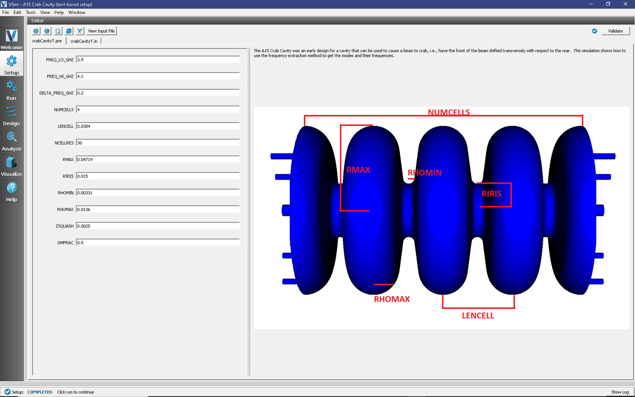
Fig. 385 Setup Window for the Crab Cavity example.

Input File Features

The input file allows the user to control a number of features of the Crab Cavity simulation. The FREQ_LO_GHZ and FREQ_HI_GHZ defines the range of frequencies that we are interested in extracting whereas the DELTA_FREQ_GHZ specifies the separation in frequency between the range of interest and the next nearest mode (at 4.3 GHz).

The input file is written to run for a long time, sufficient to ring up the cavity, then dump periodically during the free oscillation period. The modes and frequencies will be extracted from those dumps. This can be seen in crabCavityT.in.

The remaining key parameter values correspond to the geometry and discretization of the cells. The focus of the Crab Cavity simulation is on a four cell cavity with end holes that were originally used for measurement purposes. See [2]. The final ZSQUASH parameter is used to squeeze each cell of the cavity to eliminate the degeneracy due to cylindrical symmetry.

Running the Simulation

After examining the inputs, do the following:

• Proceed to the Run Window by pressing the Run button in the left column of buttons.

• Select running in parallel as desired.

• To run the file, click on the Run button in the upper left corner of the Logs and Output Files pane on the right. You will see the output of the run in this pane. The run has completed when you see the output, “Engine completed successfully.” This is shown in Fig. 386.

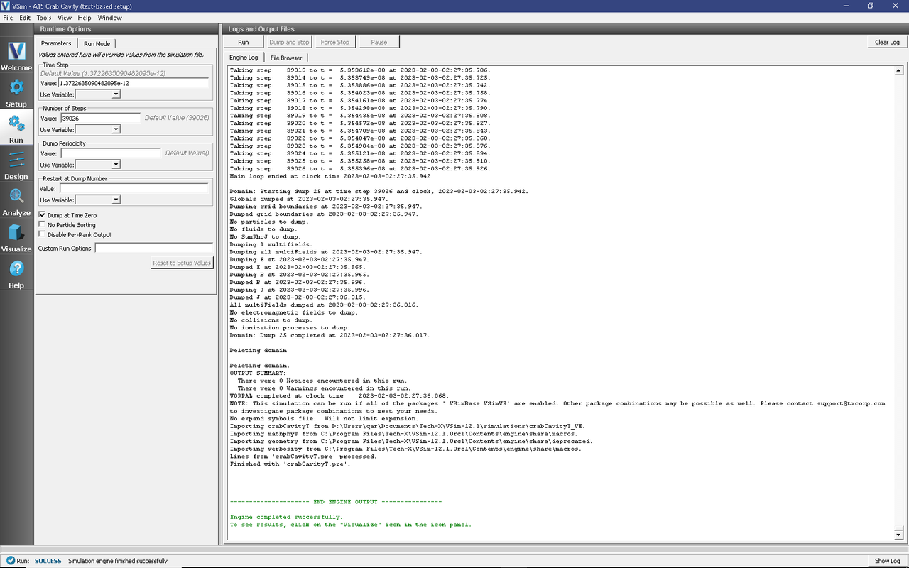
Fig. 386 The Run Window at the end of execution.

Analyzing the Results

It is possible to extract the modes of the A15 crab cavity via post processing using the Extract Modes Analysis Script* as follows:

• Press the Analyze button in the left column of buttons.

• From the list of Available Analyzers, select extractModes.py and press Open.

• Enter the following parameters in the appropriate fields. the default simulation values are used:

  • simulationName = crabCavityT

  • field = B

  • beginDump = 2

  • endDump = 22

  • nModes = 5

  • numberUniformPts = 20

  • numberRandomPts = 20

• Uncheck the randomSample box, and check the construct box.

• Click the Analyze button in the upper right corner of the window.

As shown in Fig. 387 below, three columns of data with the titles “freq [Hz]” (eigenmode frequency), “invQ” (inverse quality factor), and “SVD” (singular value decomposition) will be output in the right pane. The analysis has completed when you see the output “Analysis completed successfully.” One can see 5 modes, but the first one is not real as one can see from its unrealistic value of invQ, which should in fact be zero for this ideal (non-lossy) cavity, and the fact that it has zero frequency.

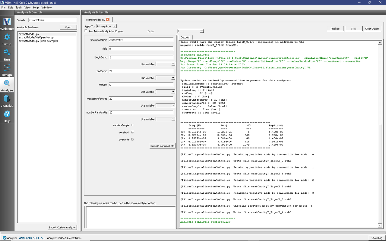
Fig. 387 The Analysis window at the end of execution of the extractModes.py script.

The magnetic fields at each of the eigenmode frequencies will be available to view in the Visualize Window under the B Field.

Visualizing the results

After performing the above actions, continue as follows:

• Proceed to the Visualize Window by pressing the Visualize button in the left column of buttons.

To view the electric field:

• Expand Scalar Data

• Expand E

• Select E_z

• Check the Clip Plot box

• Expand Geometries

• Select poly

• Check the Clip Plot box

• Move the slider at the bottom of the right pane to see the electric field at different times.

One can instead view the eigenmodes, which are so labeled under B. E.g., Unclick E_z click B_y (Eigenmode). For these plots you may want to individually control the field colors. This is done by while you have B_y (Eigenmode) selected.

Check the *Set Minimum box and set the value to -0.005 Check the *Set Maximum box and set the value to 0.005

This will give a sharper contrast of the eigenmode The slider can be moved to see the eigenmodes, as it is used for the mode number rather than periods in time. Slider positions past the last eigenmode will display only the last eigenmode.

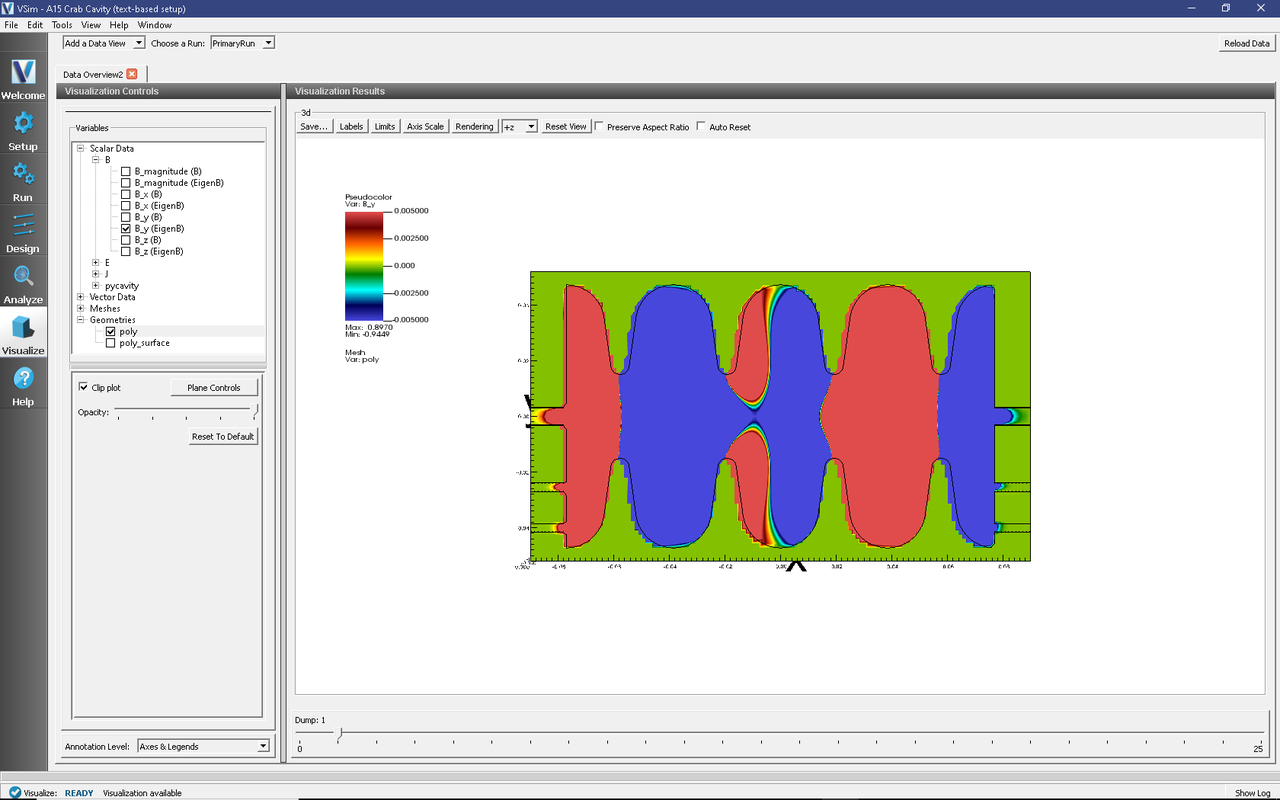
Fig. 388 Visualization showing an eigenmode

Further Experiments

Additional experiments worth investigating are:

• Use Histories to record the power flow, to compute the coupling efficiency.

• Simulate one period of the waveguide with periodic boundary conditions and a user-defined phase shift, and use the frequency extraction feature to compute the waveguide modes and dispersion curves.

References

[1] G. R. Werner and J.R. Cary, “Extracting modes and frequencies from time-domain simulations with filter-diagonalization”, J. Comp. Phys., 227 (10), 5200-5214, 2008.

[2] T. M. Austin et al., “Validation of frequency extraction calculations from time-domain simulations of accelerator cavities”, Comput. Sci. Disc., 4, 015004, 2011.