Circular Metal Waveguide Dispersion (circMetalWaveguideDisp.sdf)

Keywords:

Waveguide, Dispersion Relation, Fourier Transform, Phase Shifting Boundary Conditions

Problem description

This XSimEM example demonstrates several unique capabilities of XSim that can be used to efficiently model waveguides. One unique capability is the use of phase shifting periodic boundary conditions. These work by adding a phase to a wave at a boundary to mimic a much longer physical dimension. We also demonstrate how to use an analyzer called extractModesViaOperator.py to accurately compute the excited modes in the waveguide, even if some of the modes are much weaker than the dominant mode. In this example, we use extractModesViaOperator.py to compute the dispersion relation (\(\omega\) vs \(k\)) and compare the numerically determined dispersion relation with the theoretical dispersion relation using standard waveguide theory.

This example involves five steps. In the first step, the waveguide is “pinged” with a short pulse in the current density that excites a range of modes. The Fourier transform then shows the range of frequencies of the modes. In the second step, the waveguide is excited using a sinc pulse function multiplied by a Gaussian envelope to excite a flat band of frequencies with sharp cutoffs at either end. The excitation current density is in the transverse directions (\(z\) and \(y\)) which excites an electric field primarily in the transverse direction. In the third step, the data is restarted from the end of the second run and saved at shorter time intervals in order to resolve the frequencies of interest. The output from the third step is used by the extractModesViaOperator.py analyzer to compute the eigenmodes in step 4. Finally, in step 5, the dispersion relation is computed by varying the wavelength which is resolved in the simulation.

Opening the Simulation

The circular metal waveguide dispersion example is accessed from within XSimComposer by the following actions:

• Go to File → New → From Example…

• In the resulting Examples window expand the XSim for Electromagnetics option.

• Expand the Cavities and Waveguides option.

• Select “Circular Metal Waveguide Dispersion” and press the Choose button.

• In the resulting dialog, create a New Folder if desired, and press the Save button to create a copy of this example.

The properties and values that create the simulation are accessible in the left pane when the Setup Window is selected as shown in Fig. 338. The right pane shows a 3D view of the selected geometry components, grids and current distributions.

The geometry can be visualized by expanding “Geometries” in the left pane. The hollow circular waveguide can be seen more clearly by de-selecting the “Grid” option. The length in the direction of propagation (\(x\)) is a small fraction of either transverse direction. This is possible because we are using “phase shifting periodic” boundary conditions in the x -direction. The phase shifting BCs are selected under “Basic Settings”.

A sinc hat function is used to excite the waveguide.

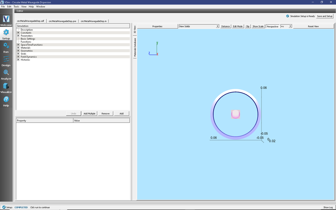
Fig. 338 Initial Setup Window for the Waveguide Dispersion example. The block in the middle is the region in which the current density is driven.

Phase Shifting Boundary Conditions and Phase Shift

Before discussing phase-shifting periodic boundary conditions, we first review ordinary periodic BCs. In this discussion, periodic BC’s are applied in the x-direction. With normal periodic BC’s, there are two criteria in resolving a wave (or mode) of interest. (1) There must be enough grid points along the wavelength to resolve the spatial profile. Typically we sample at least 20 cells along a wavelength (\(\lambda_x\)), or \(DX = \lambda_x/20\), and (2) The length of the simulation domain, represented by \(L_x\), must be one wavelength long, \(L_x=\lambda_x\). Periodic BC’s in the x-direction means that \(F(0)=F(L_x)\), where \(F\) is any field quantity. Now introduce a grid that extends from 0,1,…,nx and let \(x=0\) at grid point 0 and \(x=L_x\) at grid point nx. Periodicity on the grid implies \(F(0)=F(nx)\). Finally, let’s assume that \(F(x)\sim \sin(k_x x)\). Then, applying the condition for periodicity, \(\sin(0) = \sin(k_x L_x)\), which is exactly met if \(L_x=\lambda_x\).

With phase-shifting periodic BC’s, we are no longer required to meet the second criteria discussed in the preceding paragraph. To see this, let’s suppose that \(L_x < \lambda_x\). Then the periodicity condition can still be met by setting \(k_x L_x - \phi_0=0\), where \(\phi_0\) is the phase shift equal to \(k_x L_x\), which is the exact phase shift we have chosen to apply in XSim for this example. The numerical implementation is more challenging than the conceptual picture we just discussed. To implement phase-shifting periodic BC’s, we need to treat the fields as complex numbers and set \(F(L_x)=\exp(i \phi_0)F(0)\). For the grid, we pick 2 cells such that \(L_x=2DX\).

By using phase-shifting periodic BC’s, we can simulate different physical lengths without changing the simulation length \(L_x\) through the phase shift \(\phi_0=k_x L_x\). Because \(k_x=2\pi/L_x\), we can solve for \(\omega(k_x)\) without requiring a simulation of length \(L_x\).

Running the Simulation and Analyzing Results

We now walk through the five steps discussed in the Introduction. In the first step, we test to determine the minimum frequency that will propagate through the waveguide. For the circular waveguide in this example, we know the analytical result which is the lowest cutoff frequency. However, we still do this step to demonstrate how to determine the lowest frequency that will propagate for cases that are not analytic. In the second step, the current density “rings up” to a maximum value, then rings down to 0. Because we are exciting modes at resonant frequencies of the cavity, the E- and B-fields continue to oscillate after the excitation is turned off. We wish to determine the resonant modes using Eigen mode analysis using data saved in Step 3 when the externally driven source is turned off and the cavity is “ringing” at its natural frequencies. In step 4, extractModesViaOperator.py is used to compute the excitation frequencies in the cavity at a given mode. Finally, in step 5, you will change the value of “mode”, which is defined under “Constants” to compute the dominant frequencies which are excited in the cavity at a given wavelength. We assume the maximum wavelength which can be resolved in a traditional periodic simulation is 0.2 m and denote this as lambdaMax. We then define the parameter \(k_x=\frac{mode}{12}\frac{2\pi}{lambdaMax}\) and run 25 simulations with mode =0,1,2,…,24. Finally, we set the phase shift to \(k_x \times L_x\) to ensure the correct phase shift is applied for the phase shifting periodic BC’s. In this way, we are able to compare the simulation with waveguide theory without explicitly changing the length of the simulation domain in the x -direction.

Step 1: Determining the lowest cutoff frequency - The “Ping” Run

The Ping run is used to determine the lowest propagation frequency in the waveguide. In this simulation, we can analytically compute the lowest propagation frequency at a given k based on the allowable modes in a circular wave guide. We can then compare the computed lowest propagation frequency with theory. However, for arbitrarily-shaped waveguides, this step is necessary since no theory is available to compute the lowest propagation frequency. We have defined two constants in order to easily transition from the “Ping” run to the “Excitation” run in Step 2. For Step 1, perform the following steps

• Go to the Setup Window and expand the Constants option

• Set PINGON to 1

• Click on Save and Setup in the upper right corner of the visualization window

• Click on the Run button.

• Set Number of Steps to 5000

• Set Dump Periodicity to 1000

• This simulation may be accelerated by changing the Run Mode to Parallel

• Click the Run button on the upper left corner of the Logs and Output Files pane

The run has completed when you see the output, “Engine completed successfully.” A snapshot of the simulation run completion is shown in Fig. 339.

Fig. 339 The Run window at the end of a Step 1.

After the run has completed, click on the Visualize tab on the left side of the visualization window. After the data has loaded, click on Add a Data View and then select History. Perform the following steps to analyze the history:

• Graph 1 select jMid_1

• Graph 2 select eMid_1

• Graphs 3 and 4 select none

In Graph 1, to see the data, click on the “Limits” option above the plot. Set the X-axis upper limit to 2e-10. You should see a step function in the current density beginning at t=0 and ending abruptly after about 20 time steps. This is the “ping” that we impose on the simulation. To determine the lowest frequency mode that we excite, click the “Fourier Amplitudes (dB)” box in Graph 2. Again, click on the “Limits” button above and to the right of the graph. Set the X-axis upper limit to 4e9. You will see that the first peak occurs at a frequency of about \(1.75\times 10^9\) Hz, which is the lowest cutoff frequency in the simulation and is what we find analytically using waveguide theory. Therefore, we have confirmed that XSim reproduces linear theory. You can confidently use XSim to numerically determine the lowest cutoff frequency for non-analytically solvable shapes. The visualization window after the above steps have been performed is shown in Fig. 340

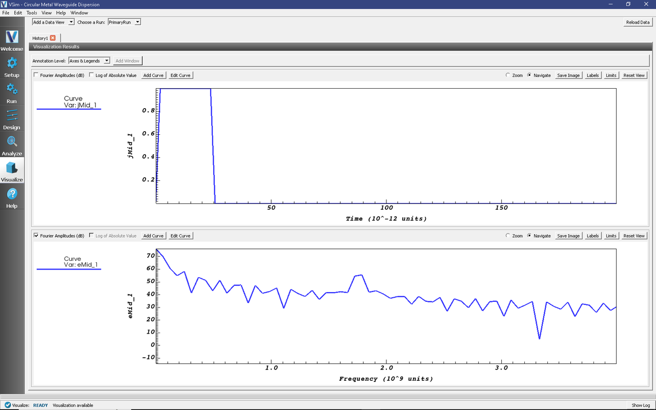
Fig. 340 History plots showing the lowest cutoff frequency at \(1.75\times 10^9\) Hz as the result of pinging the waveguide with an abruptly applied current density.

Step 2: Excitation

From Step 1, we know that the lowest propagation frequency is \(\sim 1.75\times 10^9\) Hz. We can now check that the lowest cutoff frequency (frequency low in SincHat) is correct. The parameter FREQ_MIN is passed into frequency low in the SincHat function and is indeed \(\sim 1.75\times 10^9\) Hz. We can now proceed to excite the waveguide with confidence knowing that lowest excitation frequency is correct. To excite the waveguide, perform the following steps:

• Go to the Setup Window and expand the Constants option

• Set PINGON to 0

• This will change the applied current to the SincHat function.

• Click on Save and Setup in the upper right corner of the visualization window

• Go to the Run Window by pressing the Run button in the left column of buttons.

• This simulation may be accelerated by running on multiple MPI ranks. The parallel options are in the Run Mode tab

• The default run options are set up in “Basic Settings” in the Setup Window. We are dumping in groups of 3. For the data to be saved in groups of 3 the Dump Periodicity must be left blank. However, in the second step, we do not want to dump in groups of 3. Therefore, set Dump Periodicity to 1000

• Set Number of Steps to 21000. This ensures that the simulation runs long enough for the current density to “ring up” then “ring down” to 0.

• To run the file, click on the Run button in the upper left corner of the Logs and Output Files pane. You will see the output of the run in this pane. The run has completed when you see the output, “Engine completed successfully.” A snapshot of the simulation run completion is shown in Fig. 341.

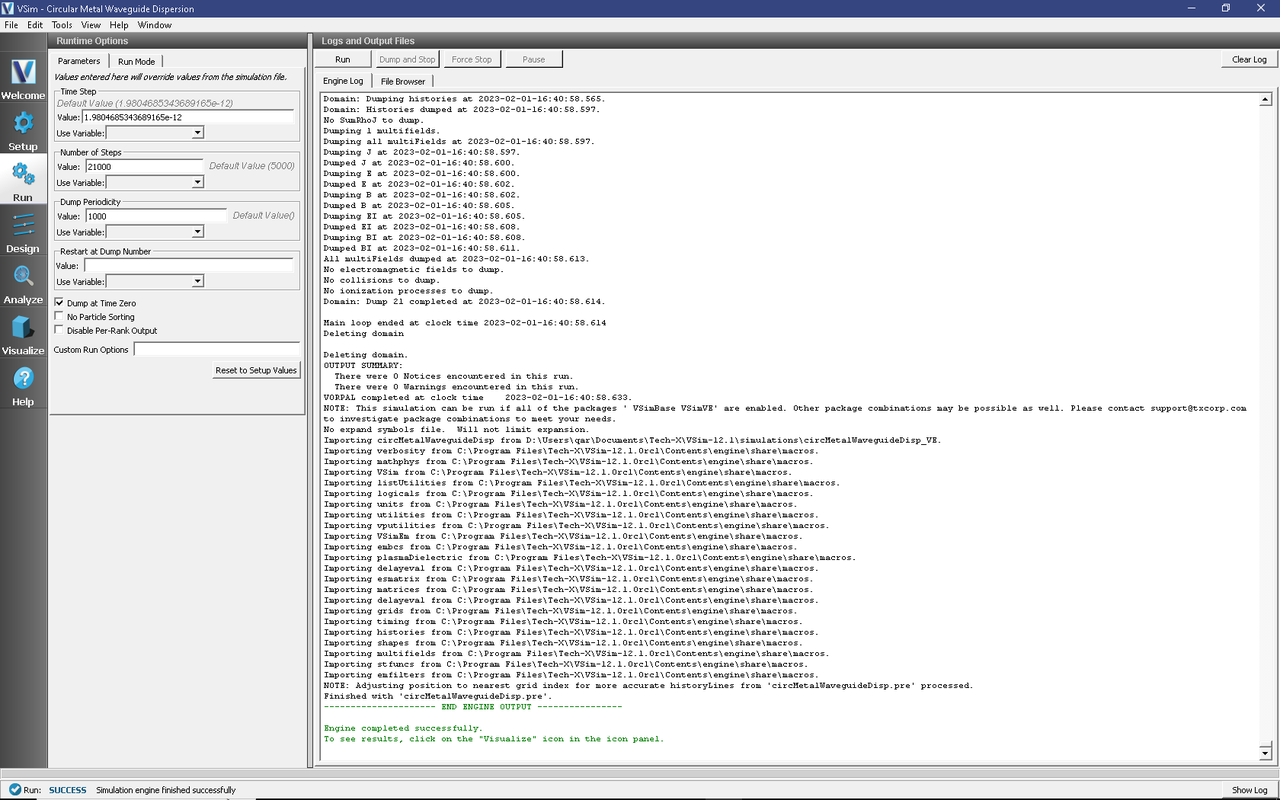
Fig. 341 The Run window at the end of a Step 2.

Step 3: Evolving the excited cavity

The purpose of Step 3 is to continue the simulation with only the E- and B- fields excited due to the externally imposed current density from Step 2. We will also save more data which we can analyze using Eigenmode analysis for Step 4.

• After Step 2 is complete, set the number of steps to 10000. Make sure “Dump Periodicity” is left blank. The simulation will revert to the values defined in “Basic Settings” which are dump every 100 time steps in groups of 3 (10100,10101,10102, …, 10200,10201,10202,…, etc). If you fill in an integer into Dump Periodicity, the default gets overwritten and the data are not dumped in groups of 3, which is required for the extractModesViaOperator.py analyzer.

• In the Additional Run Options Box, make sure that the Dump at Time Zero box is unchecked and that Restart at Dump Number is set to 21.

• Click run. The run has completed when you see the output, “Engine completed successfully.” A snapshot of the simulation run completion is shown in Fig. 342. When this run is finished, the last step should be step 31000.

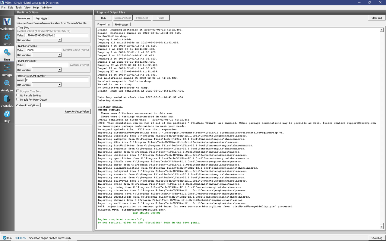
Fig. 342 The Run window at the end of Step 3.

Step 4: Computing the eigenmodes

• Go to the analyzer window by selecting Analyze in the left column.

• Select extractModesViaOperator.py from the list of available analyzers. Then click “Open” on the top right of the Analysis Controls pane.

• Compute the electric field eigenfunctions. After the analyzer loads, ensure the following parameters are entered:

  • simulationName: “circMetalWaveguideDisp”

  • outputsimName: leave blank

  • realFields: “E”

  • imagFields: leave blank

  • secondFieldFactor: leave blank

  • operator: “d2dt2”

  • dumpRange: “21:321”

  • cellSamples: “:,5:55:5,5:55:5”

  • cutoff: “1e-12”

  • maxNumModes: “-1”

  • initialModeNumber: “0”

  • normalizeModes: checked

  • testing: leave blank

  • compMajorC: leave blank

  • overwrite: checked

The dump range runs only over the data saved in step 3 and we are only sampling every 5 cells in the z- and y- directions which is adequate to compute the eigen modes. Double-check your entries against what is shown in Fig. 343. After you run the analyzer, you will need to scroll up to find the computed frequencies. The screenshot shown in Fig. 343 is from a visualization window that is scrolled up so that the computed frequencies can be compared with what you ran. Figure Fig. 343 shows that there are 6 unique modes. One indication that you are using extractModesViaOperator.py correctly is that the imaginary part of the frequency (which represents attenuation of the wave) is nearly 0 or at least much smaller than the real part. The lowest excited mode is \(\sim 1.76 \times 10^9\) Hz, which is discussed further below in the context of standard waveguide theory.

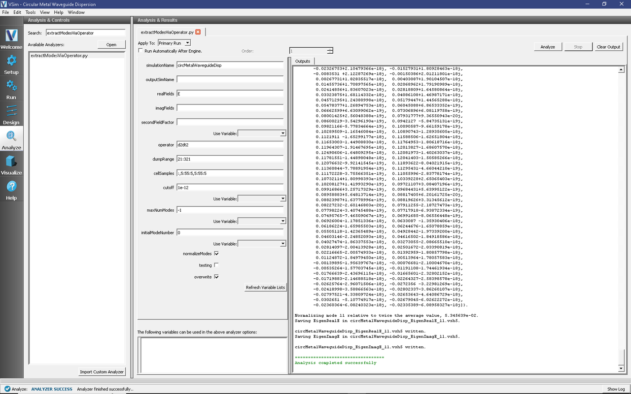
Fig. 343 Computing the electric field eigenfunctions and frequencies using the extractModesViaOperator.py analyzer.

Step 5: Computing the Dispersion Relation

Once the Eigenmode analysis is complete in Step 4, it is necessary to record the three lowest-order modes. The pre-loaded value of mode is 1, which means we are simulating \(k_x=\frac{1}{24}\frac{2\pi}{\lambda}\), where \(\lambda=0.2\) m. Also, the waveguide dispersion relation is given by \(\omega^2 = k_x^2 c^2 + \omega_{mn}^2\), where \(\omega_{mn}^2 = \frac{c^2}{R^2}(x'_{mn})^2\), where m and n are integers and \(x'_{mn}\) is the nth root of \(J'_m(x)=0\) (the derivative of the cylindrical Bessel function of the first kind). The first three allowable modes are \(x'_{11}\approx 1.841, x'_{21}\approx 3.054\) and \(x'_{01}\approx 3.832\). Furthermore, the frequency range that is excited lies between \(f_l = 1.75\times 10^9\) Hz (which is the lowest allowable propagation frequency) and \(f_h = 5.2\times 10^9\) Hz. Given these parameters, we expect from waveguide theory for the three lowest modes to be \(\sim 1.76\times 10^9, 2.92\times 10^9, 3.66 \times 10^9\) Hz, which is what is found from extractModesViaOperator.py. Repeating these steps for modes 1 to 24 yields the dispersion relation shown in Fig. 344. The overlap between the simulation results and theoretical values is evident in Fig. 344.

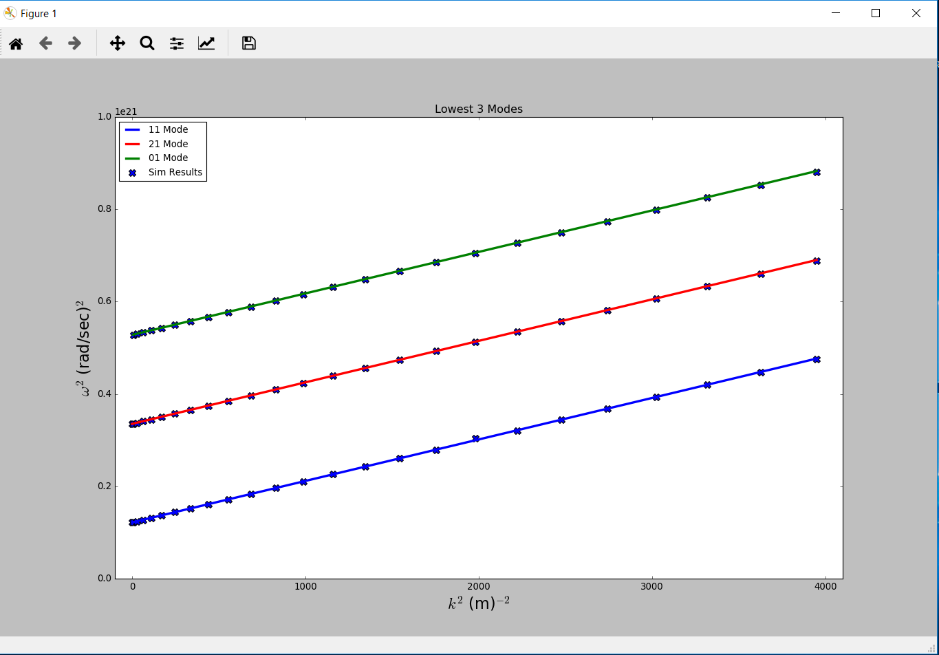
Fig. 344 Dispersion relation found by changing mode in XSim. The solid line is theoretical dispersion relation \(\omega^2 = k_x^2 c^2 + \omega_{mn}^2\). The ‘X’s represent data from the simulation results.

Convergence Study

To demonstrate that the simulation results converge to the theoretical value, we have performed a series of simulations in which \(DX=DY=DZ\) are varied. The values chosen are DX = 0.25, 0.33, 0.5 and 0.733 cm. We then computed the lowest propagation frequency using extractModesViaOperator.py and plotted this frequency versus \(DX^2\). Using Richardson extrapolation, we then compute the lowest propagation frequency for \(DX^2=0\), which provides a better comparison with the theoretical frequency than a simulation with finite \(DX^2\). The field calculation error scales approximately with \(DX^2\) so a plot of frequency versus \(DX^2\) should be a line. The linear correlation between frequency and \(DX^2\) is shown in Fig. 345. The extrapolated frequency at \(DX^2=0\) is \(\sim 1.75686 \times 10^9\) Hz. The theoretical value is \(\sim 1.75681 \times 10^9\). Therefore, we see from Fig. 345 that the computation of the lowest propagation frequency for the DC mode converges with order \(DX^2\), which is expected since the field solve is 2nd order accurate. Furthermore, using Richardson extrapolation, we see that the difference between theory and simulation, with \(DX^2=0\), is \(0.003\) %.

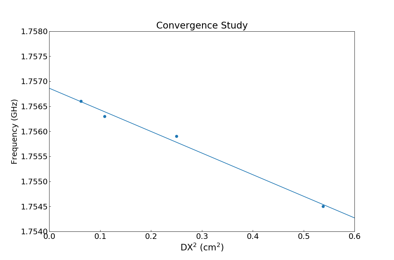
Fig. 345 Plot demonstrating convergence of frequency calculation.

Visualizing the results

After performing the above actions, continue as follows:

• Proceed to the Visualize Window by pressing the Visualize button in the left column of buttons.

• Click on Reload Data

The first step will be to ensure that we are driving the current density as expected and that the E- and B- fields are “ringing” as a result of driving the current density. Follow these steps to perform this check:

• Click on the Add a Data View pull-down menu at the top of the visualization window

• Click on History. This will open a new tab.

• Under Graph 1 plot jMid_1. This is the y- component of the current density

• Under Graph 2 plot eMid_1.

• Under Graph 3 plot eMid_2.

• Under Graph 4 plot bMid_0.

Your plots should be similar to Fig. 346. The current density is driven for a short time period. However, because we are driving resonant modes, the current density excites the transverse electric field and parallel magnetic field. You can also plot eMid_0 to compare with Fig. 346. Since eMid_0 is ~ 0, we are driving a TE waveguide.

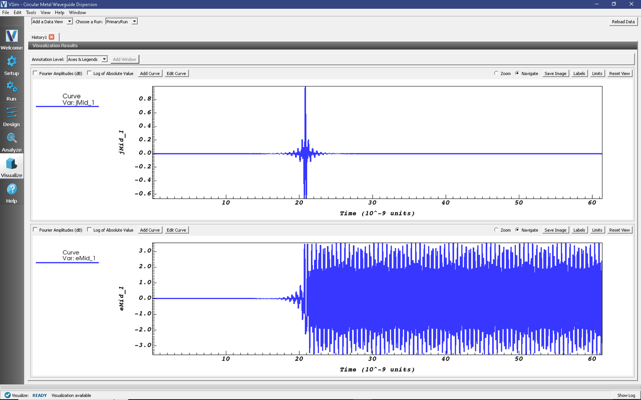
Fig. 346 History plots showing the modes driven in this simulation

We next wish to examine the spectral characteristics of the current density, which is driven between FREQ_MIN and FREQ_MAX. Therefore, the Fourier Transform of \(J_y\) or \(J_z\) should be greatest in this frequency range. Returning to the History visualization window, under Graphs 2, 3, and 4, change the plotted quantity to none, so that only Graph 1 shows a plot. Now check the “Fourier Amplitudes (dB)” box in the upper left corner. Finally, check the “Zoom” box on the right side of the visualization window and highlight from 0 to \(10^{10}\) Hz which will expand the lower frequency part of the plot. After you have zoomed in on the plot, re-check the “Navigate” box. The result of these steps should lead to a plot that looks similar to Fig. 347. The driving frequencies lie between FREQ_MIN and FREQ_MAX as expected. The rate at which the Fourier signal dampens below FREQ_MIN and above FREQ_MAX depends on the Gaussian envelope and the parameter called OMEGA_SIGMA.

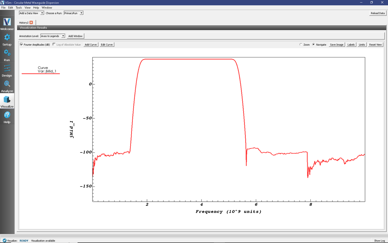
Fig. 347 Fourier Transform of the current density showing that the current density is mainly driven between FREQ_MIN and FREQ_MAX as expected.

Further Experiments

The result of varying mode from 0 to 24 is shown in Fig. 344. One experiment you can perform is to reproduce Fig. 344 by running 25 simulations with mode varying from 0 to 24. Each simulation takes just a few minutes so the 25 simulations takes about one hour. For each simulation record the three lowest frequencies that are excited using extractModesViaOperator.py.

Another experiment would be to change the dimensions of the waveguide. The constant InnerRadius is used to determine the lowest frequency that will propagate in the waveguide. Therefore, changing InnerRadius will automatically compute FREQ_CUTOFF_TE. You will then need to change BGNY, ENDY, BGNZ, and ENDZ so that the primitive fits within the simulation domain. The primitive geometry called “pipe0” scales with the constant InnerRadius.

A third experiment would be to modify FREQ_MIN and FREQ_MAX and compute the dispersion curve for these new values. No mode will propagate below FREQ_CUTOFF_TE so do not set FREQ_MIN below FREQ_CUTOFF_TE.

Lastly, you can try to propagate a TM mode instead of a TE mode.