Coaxial Cylinder (coax.sdf)
Keywords:
- coax, coaxial geometry, cylinder, current pulse, rlc circuit, step potential
Problem description
This example probes the electromagnetic properties of a semi-infinite coaxial cylinder. One end of the cylinder lies in the simulation space. The length of the cable is large compared to its diameter. The outer radius is 8 cm, the inner radius is 2 cm, and the section considered is 20 cm long. The inner cylinder is shorter than the outer cylinder and there is an electron absorbing cap on the end of the outer cylinder. When the simulation initiates, a single EM pulse is launched into the open, continuous end of the geometry and propagates to the capped tip. Electrons are ejected from the tip of the inner cylinder when the pulse reaches it.
This computational model is equivalent to applying a step-potential to one end of a coaxial cable. The step-potential propagates at the speed of light until it reaches the tip of the inner cylinder. The RLC nature of the coax cable causes overshoot and ringing of the potential. At the inner tip, an attenuating series of oscillations occurs accompanied by electron emissions. Gradually the tip potential stabilizes at the applied potential.
This simulation can be performed with a VSimVE license.
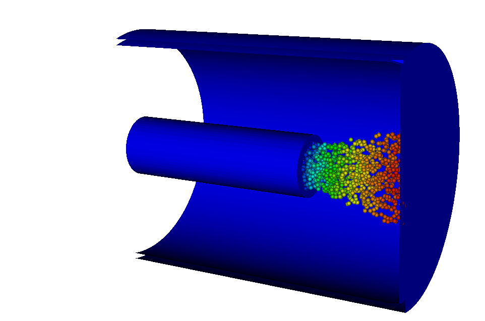
Fig. 348 The electrons are emitted from the tip of the inner cylinder after the pulse reaches it.
Opening the simulation
The coax example is accessed from within VSimComposer by the following actions:
Select the New → From Example… menu item in the File menu.
In the resulting Examples window expand the VSim for Vacuum Electronics option.
Expand the Cavities and Waveguides option.
Select Coaxial Cylinder and press the Choose button.
In the resulting dialog, create a New Folder if desired, and press the Save button to create a copy of this example.
All of the properties and values that create the simulation are now available in
the Setup Window as shown in Fig. 349. You can expand the tree
elements and navigate through the various properties, making any changes you
desire. The right pane shows a 3D view of the geometry, if any, as well as the
grid, if actively shown. To show or hide the grid, expand the Grid element and
select or deselect the box next to Grid.
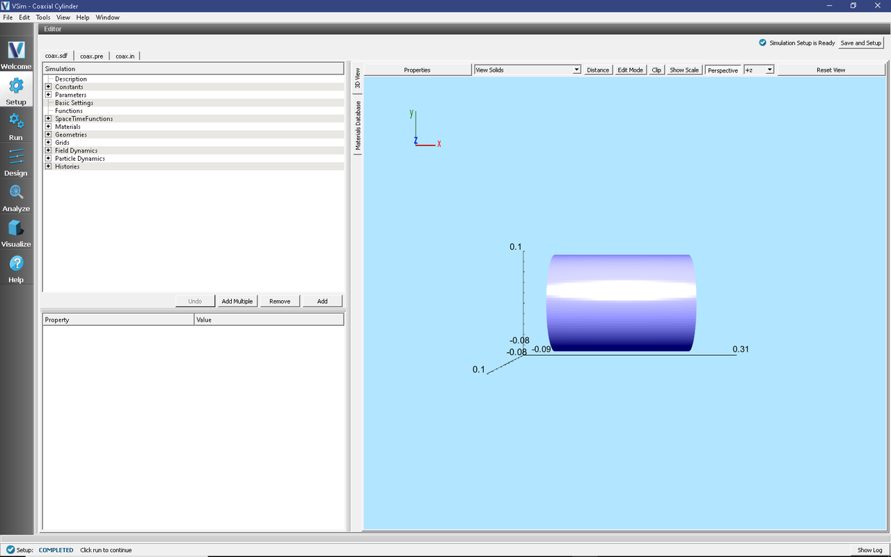
Fig. 349 Setup Window for the Coaxial Cylinder example.
Simulation properties
The coax example includes several Constants for easy adjustment of simulation properties. Those include:
TFACTOR: A ramping factor of the applied field
EFACTOR: The amplitude of the applied field
EMITTED_CURRENT: The current emitted from the tip of the inner cylinder
There are also several SpaceTimeFunctions defined for easy application to wave launchers and particle emitters. Those include:
edgeDy: The applied field in the y-direction
edgeDz: The applied field in the z-direction
nomask: This allows emission from the entire geometry of the flux emitter
Other Properties of the simulation include CSG defined geometries, a wave launcher on the lower x boundary, and a settable flux emitter on the tip of the inner cylinder.
Running the simulation
After performing the above actions, continue as follows:
Proceed to the Run Window by pressing the Run button in the left column.
To run the file, click the Run button in the upper left corner of the right pane. You will see the output of the run in the right pane. The run has completed when you see the output, “Engine completed successfully.” This is shown in Fig. 350.
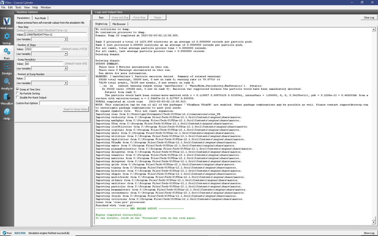
Fig. 350 The Run Window at the end of a successful execution.
Visualizing the results
After performing the above actions, continue as follows:
Proceed to the Visualize Window by clicking the Visualize button in the left column.
To create the image seen in Fig. 351, proceed as follows:
In the variables tree expand Scalar Data
Expand E
Select E_y
Click the Clip Plot checkbox
Click the Display Contours and set the # of contours to 10
Expand Geometries
Select poly (coaxGeom)
Click the Clip Plot checkbox
In the variables tree expand Particle Data
Expand electrons
Select electrons_ux
Set the size to 6
Now in the right pane move the dump slider forward in time
The axis and legends can be hidden using the dropdown menu in the lower left corner of the window
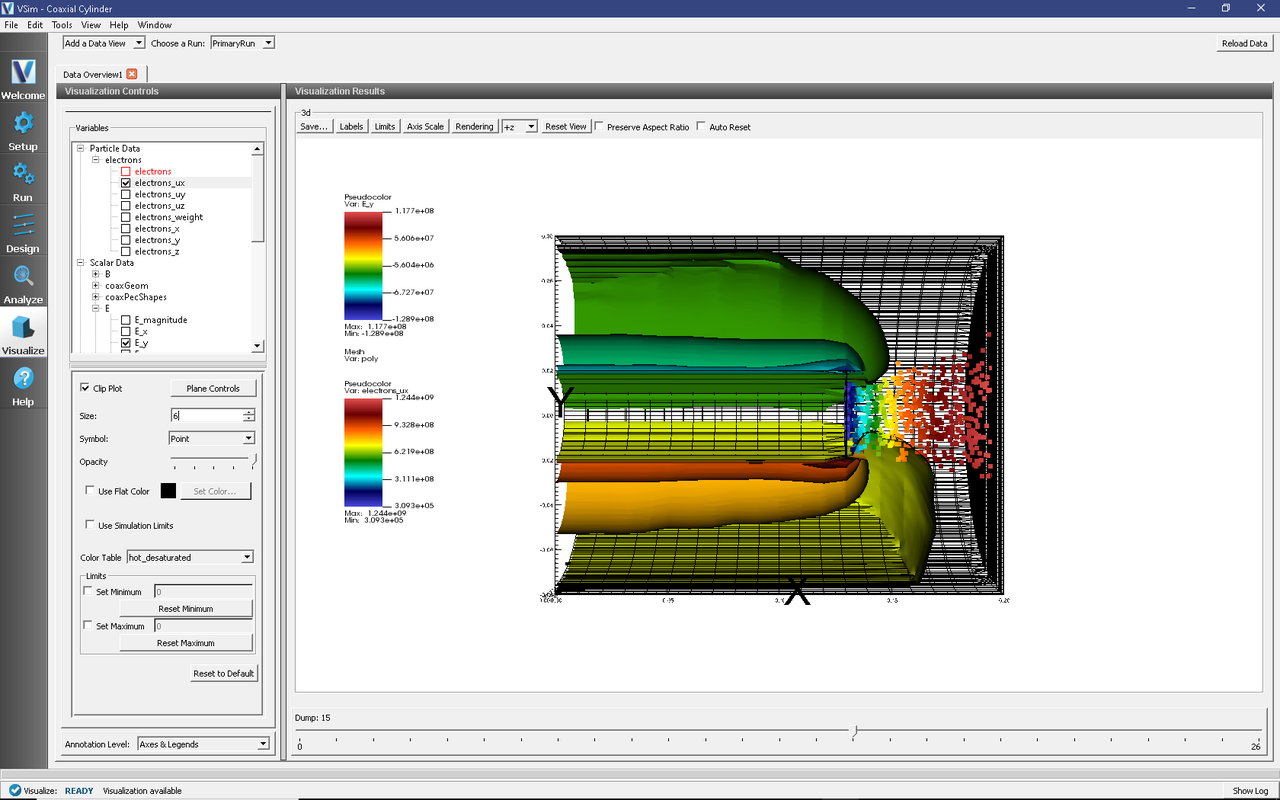
Fig. 351 Visualization of the coaxial cylinder as a color contour plot.
To obtain a clearer picture of what is happening at the cylinder tip, switch the Data View (in the left pane) to History. One dimensional plots of the number of electrons (called numMacroPtcls), the electric potential (phi), and the emitted and absorbed current should come up automatically.
You can set the location of Graph 2 to Window 1 as in Fig. 352.
The potential is measured between the interior of the inner cylinder and the capped end of the outer cylinder. The plot of the potential is noisy due to the emission of electrons from the tip. It may be insightful to run the simulation once without electrons so you can see the ringing on the waveform of phi. A similar signal is obtained by hooking up an oscilloscope to a coaxial cable. Electrons can be suppressed by setting the EMITTED_CURRENT parameter to 0 during setup.
The coaxial cylinder behaves like an RLC circuit: the cylinders provide a series resistance along their length, they are coupled capacitively, and generate self-inductance due to the current. By default, the rise-time of the pulse is near the resonance of the circuit, resulting in an acceptable rise time, low overshoot, and quick damping. This makes it a good driver of the circuit.
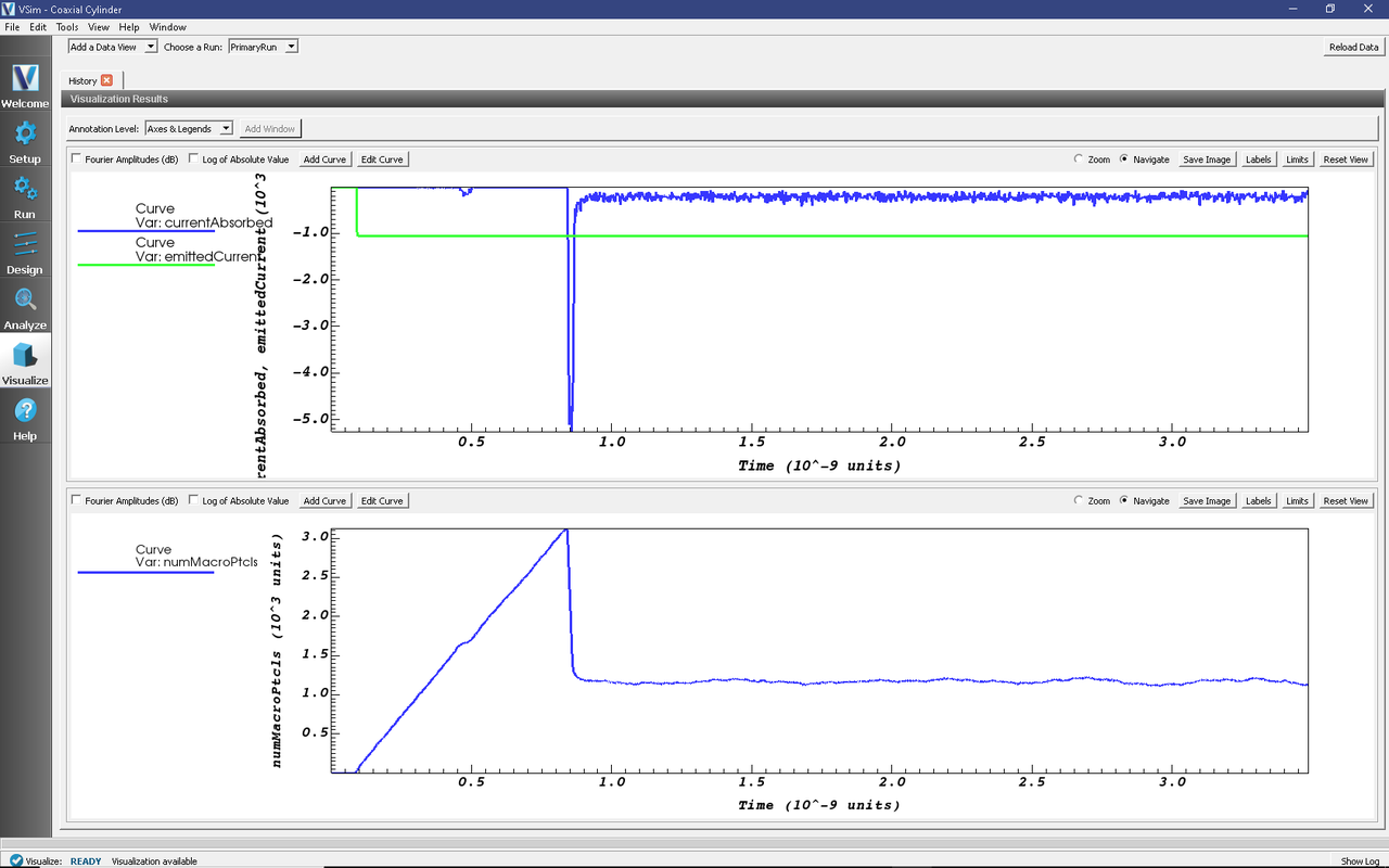
Fig. 352 The History visualization window with the electrons.
Further Experiments
Try experimenting with different dimensions of coax. In particular, note how the radii and pulse profile affect the potential response on the phi History plot.