Pillbox Cavity (pillboxCavity.sdf)

Keywords:

Pillbox cavity, Figures of merit, Transit time factor, Geometry factor

Problem description

This VSimVE example demonstrates the usage of VSim in computing the eigenmodes and figures of merit of two simple cavities. One may select either the closed pillbox cavity for which the analytic solution is well known, or a cavity based on the closed pillbox, but having outlets leading to the periodic domain boundaries. Like other examples utilizing the extractModes.py analyzer, the simulation run is done in two steps. In the first step, the cavity is excited by a sinc pulse current source and output is dumped only at the end of this excitation run. Then in the second step, output is dumped at intervals which are sufficiently short compared to the frequencies of interest. The output from the second run is used by the extractModes.py analyzer to compute the eigenmodes. Then, the computeTransitTimeFactor.py and computeCavityG analyzers are used to compute the transit time factors and geometry factors of the eigenmodes.

This simulation can be performed with a VSimVE or VSimEM license.

Opening the Simulation

The pillbox cavity example is accessed from within VSimComposer by the following actions:

• Go to File → New → From Example…

• In the resulting Examples window expand the VSim for Vacuum Electronics option.

• Expand the Cavities and Waveguides option.

• Select “Pillbox Cavity” and press the Choose button.

• In the resulting dialog, create a New Folder if desired, and press the Save button to create a copy of this example.

The properties and values that create the simulation are accessible in the left pane when the Setup Window is selected. The right pane shows a 3D view of the selected geometry components, grids and current distributions.

The geometry of the closed pillbox cavity is called pillboxCavityAnalytical and the geometry of the periodic cavity with outlets on either end is called pillboxCavityWithTube. These can be visualized individually by expanding Geometries, de-selecting and then expanding CSG, and then selecting either pillboxCavityAnalytical or pillboxCavityWithTube.

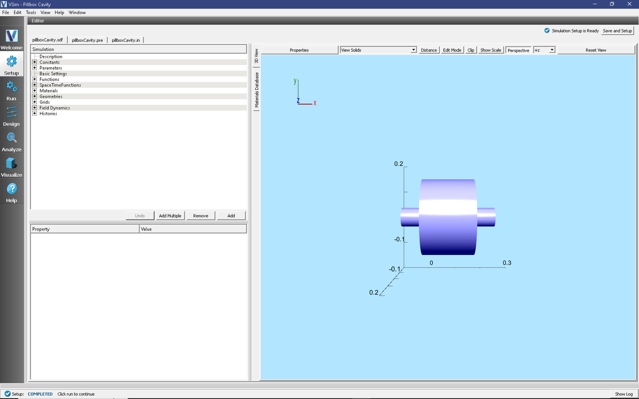
Fig. 359 Visualizing the periodic cavity geometry in the Setup Window.

Running the Simulation and Analyzing Results

Step 1: Cavity selection

• If you want to model the closed cavity, skip Step 1 and go to Step 2. The closed cavity is set by default.

• To model the periodic cavity, go to the Setup Window.

• Go to Geometries → CSG.

• Click on pillboxCavityAnalytical under CSG.

• The bottom left pane will show properties of the selected geometry. At this time, the material should be set to PEC (perfect electric conductor). Double click on PEC and select the blank line.

• Now click on pillboxCavityWithTube under CSG.

• Select PEC as the material for pillboxCavityWithTube.

Step 2: Excitation

• Go to the Run Window by pressing the Run button in the left column of buttons.

• This simulation may be accelerated by running on multiple MPI ranks. The parallel options are in the Run Mode tab

• To run the file, click on the Run button in the upper left corner of the Logs and Output Files pane. You will see the output of the run in this pane. The simulation will run for 30000 time steps and dump output once at the end. The run has completed when you see the output, “Engine completed successfully.” A snapshot of the simulation run completion is shown in Fig. 360.

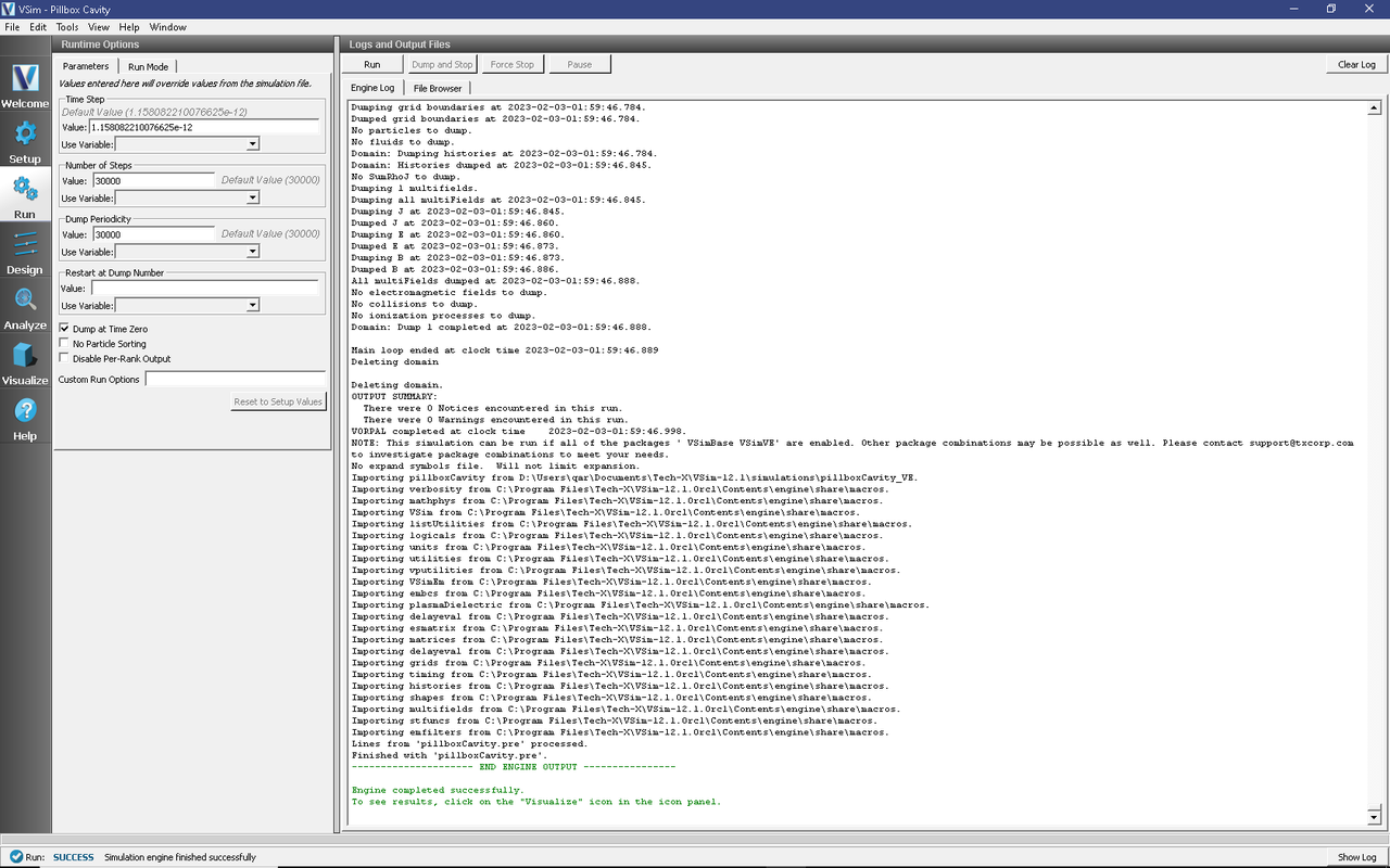
Fig. 360 The Run window at the end of a successful execution.

Step 3: Evolving the excited cavity

• After the first step is complete, change Number of Steps to 2000, change Dump Periodicity to 100.

• In the Additional Run Options Box, make sure that the Dump at Time Zero box is unchecked and that Restart at Dump Number is set to 1.

• Click run. The run has completed when you see the output, “Engine completed successfully.” A snapshot of the simulation run completion is shown in Fig. 361. When this run is finished, the last step should be step 32000.

Note

The simulation must be run in two steps because there must be no driving currents flowing in the simulation while dumping data used to extract the eigenmodes. So, while the drive is ringing the cavity, there is no need to dump data. We switch the dump periodicity after the driving current has shut off in order to resolve the frequency of the eignemodes of interest.

Fig. 361 The Run window at the end of a successful execution.

Step 4: Computing the eigenmodes

• Go to the analyzer window by selecting Analyze in the left column.

• Select extractModes.py from the list of available analyzers. Then click “Open” on the top right of the Analysis Controls pane.

• Compute the electric field eigenfunctions. After the analyzer loads, ensure the following parameters are entered:

  • simulationName: “pillboxCavity”

  • field: “E”

  • beginDump: “2”

  • endDump: “21”

  • nModes: “5”

  • sampleType: “0”

  • numberUniformPoints: “20”

  • numberRandomPoints: “100”

  • construct: “checked”

  Also, check the “Overwrite Existing Files” box. Double-check your entries against what is shown in Fig. 362.

Fig. 362 Computing the electric field eigenfunctions and frequencies using the extractModes.py analyzer.

• Press the Analyze button which is located in the upper right corner.

• Compute the magnetic field eigenfunctions with the following parameters.

  • simulationName: “pillboxCavity”

  • field: “B”

  • beginDump: “2”

  • endDump: “21”

  • nModes: “5”

  • sampleType: “0”

  • numberUniformPoints: “20”

  • numberRandomPoints: “100”

  • construct: “1”

  After the analysis is finished, and scrolling down in the Outputs log pane you should see what is shown in Fig. 363.

• Note that extractModes.py outputs the frequencies of the computed modes in the Run Output pane. The first mode, mode 0, should have a frequency of approximately 1 GHz.

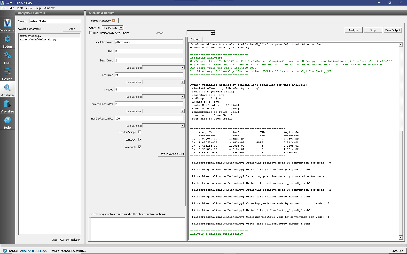
Fig. 363 The Outputs pane after Analyzing to determine the eigenmodes of the magnetic field.

Step 5: Computing the transit time factor

• Select computeTransitTimeFactor.py from the available analyzers and press “Open” on the top right of the Analysis Controls pane.

• After the analyzer loads, ensure the following parameters are entered:

  • simulationName: “pillboxCavity”

  • beginDump: “0”

  • endDump: “0”

  • beta: “1”

  • axis: “0”

  • offsetx0: “0”

  • offsetx1: “0”

  And compare against what is shown in Fig. 364

• Press Analyze.

• If you have selected the closed cavity, the transit time factor (the value following “Transit time factor, T=Vacc/V0 =”) should be very close the analytic value of \(2/\pi\).

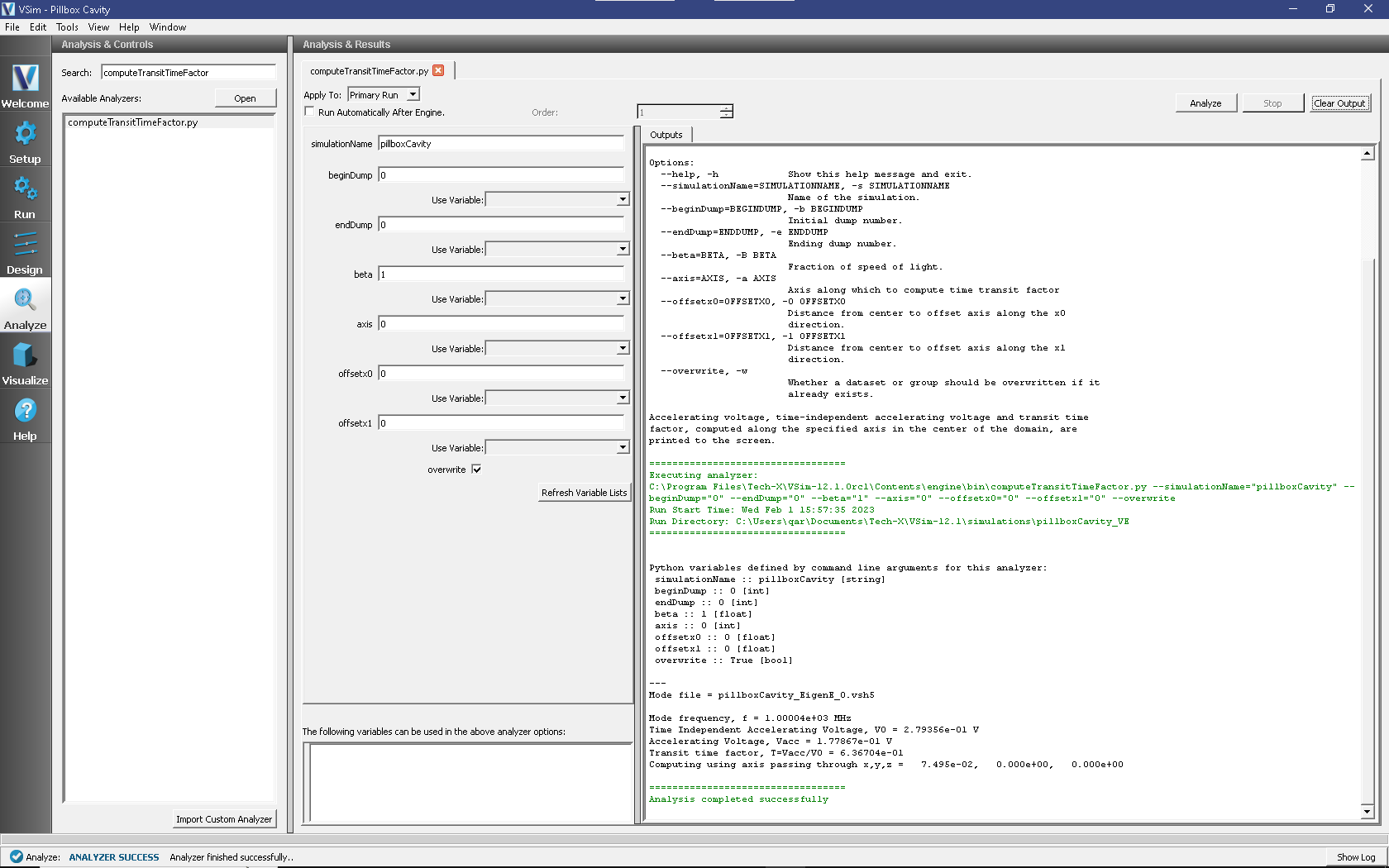
Fig. 364 Computing the transit time factor for the eigenmode of interest.

Step 6: Computing the geometry factor

• Select computeCavityG.py and click “Open”.

• If you have selected the closed cavity, then enter “pillboxCavityAnalytical” for cavityGeometryName. Otherwise, enter “pillboxCavityWithTube” for cavityGeometryName.

• Select begin dump to 0 and end dump to 2.

• If you have selected the closed cavity, the geometry factor at the mode frequency of 999.97 MHz should be very close the analytic value of 257.

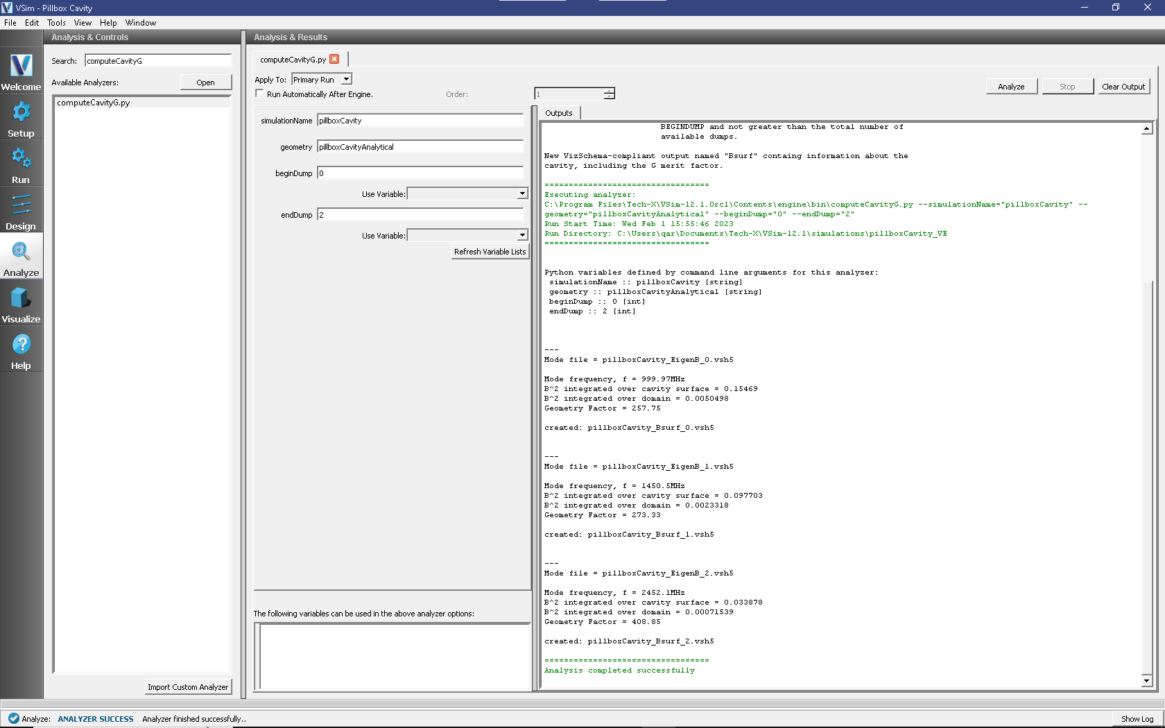
Fig. 365 Computing the geometry factor for the eigenmode of interest.

Visualizing the results

After performing the above actions, continue as follows:

• Proceed to the Visualize Window by pressing the Visualize button in the left column of buttons.

To see the projection of the magnetic field of the fundamental mode onto the cavity walls, do the following:

• Expand Scalar Data

• Expand Bsurf

• Check Bsurf_magnitude

• Click the Plane Controls button at the bottom of the Visualization Controls pane on the left of the Composer window.

• Select X as the “Clip Plane Normal” and “.05” as the “Origin of Normal Vector” for “X”. Leave the “Origin of Normal Vector” for “Y” and “Z” as 0.

• Rotate the visualization by left clicking and dragging with your mouse.

• You should see a visualization of the magnitude of the magnetic field of the fundamental mode projected onto the wall of the cavity as in Fig. 366

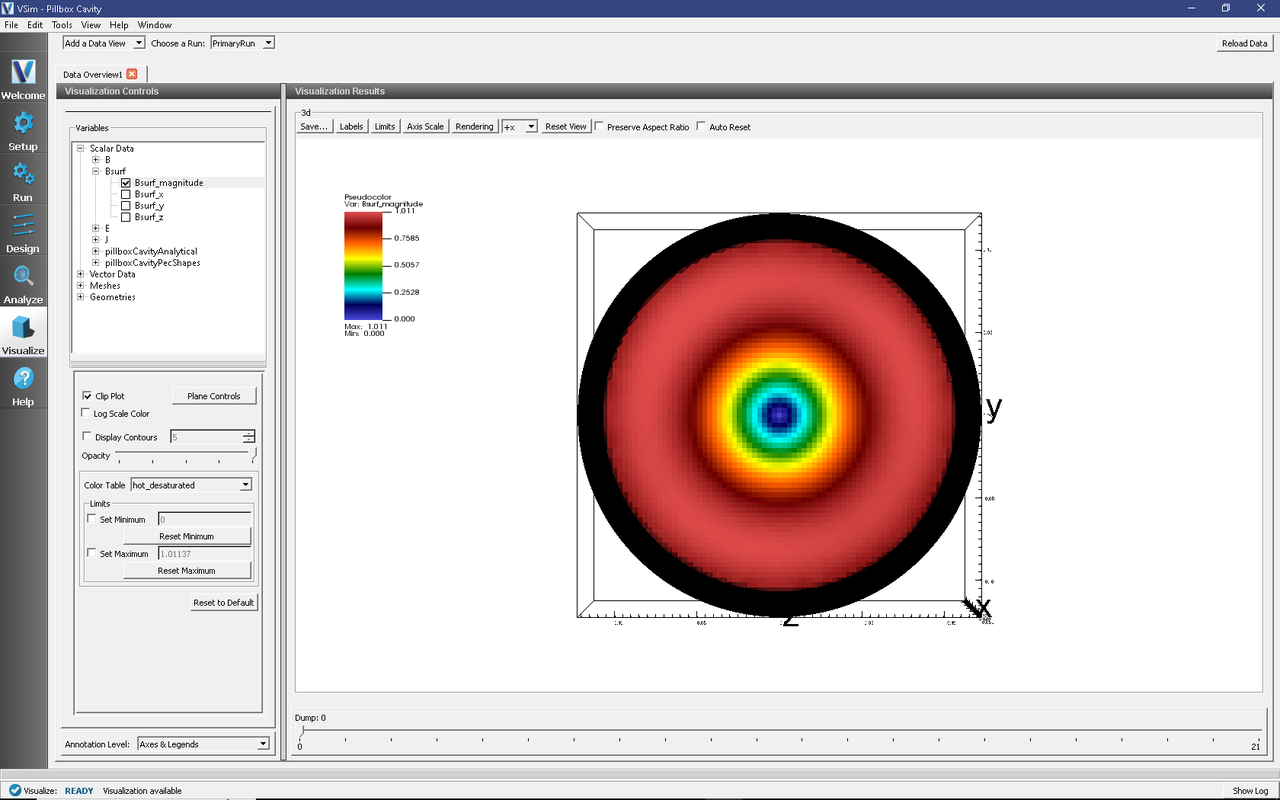
Fig. 366 The magnitude of the magnetic field on the wall of the cavity

To see a more quantitative visualization of the eigenmode fields, as shown in Fig. 367, do the following:

• Add a Field Analysis Data View

• Select the E_x (EigenE) as a field

• Under the Layout drop-down menu, select Side-by-side 2d/1d

The Bessel function dependence of the x-component of the electric field will be clearly plotted on the right.

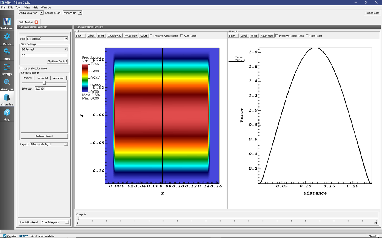
Fig. 367 Axial component of the electric field in the \(z=0\) plane (left) and plot of the axial electric field along \(z=0, x=0.07495\) (right).