Cylindrical Waveguide (cylindricalWaveguide.sdf)
Keywords:
- electromagnetics, waveguide, dispersion
Problem Description
This VSimVE example illustrates how to find the modes of a cylindrical waveguide.
This simulation can be performed with a VSimVE license.
Simulation Properties
A section of cylindrical waveguide is simulated with the goal of extracting its propagating mode frequencies. The simulation is only two cells wide in X, but through the use of a phase-shifting periodic boundary condition, a much longer waveguide is simulated. The modes are extracted for longitudinal k-vectors, \(\frac{2 \pi n}{L_x}\). The maximum current is \(I_0 = I\left(\tau/2\right)\). The waveguide is first excited with a transverse current that is off axis so as to excite modes of any symmetry. The temporal excitation is chosen to excite only a range of frequencies, from somewhat below the lowest cutoff up to the modes corresponding to \(n = 1\). The Fourier transform of a history recording the electric field shows a clean output with a modest number of modes. Precise values for those frequencies can be obtained using the extractModes analyzer.
Opening the Simulation
The Cylindrical Waveguide example is accessed from within VSimComposer by the following actions:
Select the New → From Example… menu item in the File menu.
In the resulting Examples window expand the VSim for Microwave Devices option.
Expand the Cavities and Waveguides option.
Select Cylindrical Waveguide and press the Choose button.
In the resulting dialog, create a New Folder if desired, and press the Save button to create a copy of this example.
All of the properties and values that create the simulation are now available in
the Setup Window as shown in Fig. 353. You can
expand the tree elements and navigate through the various properties, making any
changes you desire. The right pane shows a 3D view of the geometry, if any, as
well as the grid, if actively shown. (To show or hide the grid, expand the Grid
element and select or deselect the box next to Grid.) For the current
view, the setup has been rotated to be able to see down the waveguide, and the
view of the grid has been turned off. The box inside the waveguide is the
location of the current source that will drive the waveguide.
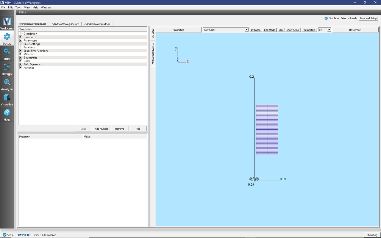
Fig. 353 Initial Setup Window for the Cylindrical Waveguide example.
The sinc hat function is used to excite this example. This function has a Fourier spectrum that is fairly flat for \(f_l < f < f_h\) and falls off rapidly over a frequency width of \(\delta_f\), so that it is nearly zero for \(f < f_l - \delta_f\) or \(f < f_h + \delta_f\). \(\delta_f\) is automatically calculated by the sinc hat function based on the suppression factor and frequency gap factor. This excitation gives a range of modes to be analyzed.
Running the Simulation
After performing the above actions, continue as follows:
Proceed to the Run Window by pressing the Run icon in the left panel.
Check the center panel that you will run for 20,000 steps, dumping every 2,000.
To run the file, click on the Run button in the upper left corner of the right panel. You will see the output of the run in the right pane. The run has completed when you see the output, “Engine completed successfully.” This is shown in Fig. 354.
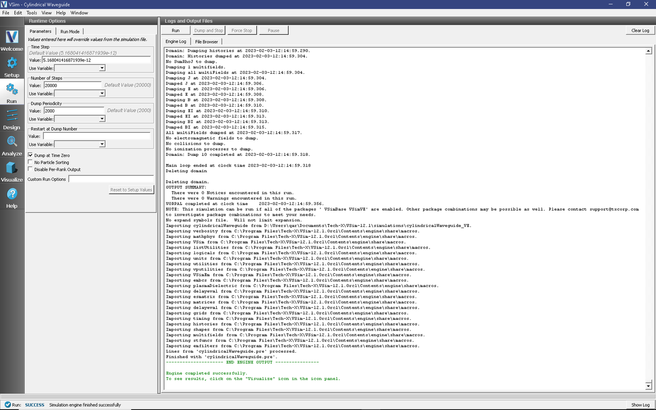
Fig. 354 Run Window for the Cylindrical Waveguide example after the initial run.
Visualizing the Spectrum
After performing the above actions, continue as follows:
Proceed to the Visualize Window by pressing the Visualize icon in the left panel.
Select History under Data View. The first History tab will have eMid_0 and eMid_1 plotted. Open a second History tab in order to plot eMid_2 as well.
Then for each plot select the Fourier Amplitude (dB) checkbox
In the upper right corner of each plot, select Limits and set X-Axis max to 2e9.
The result should be that shown in Fig. 355.
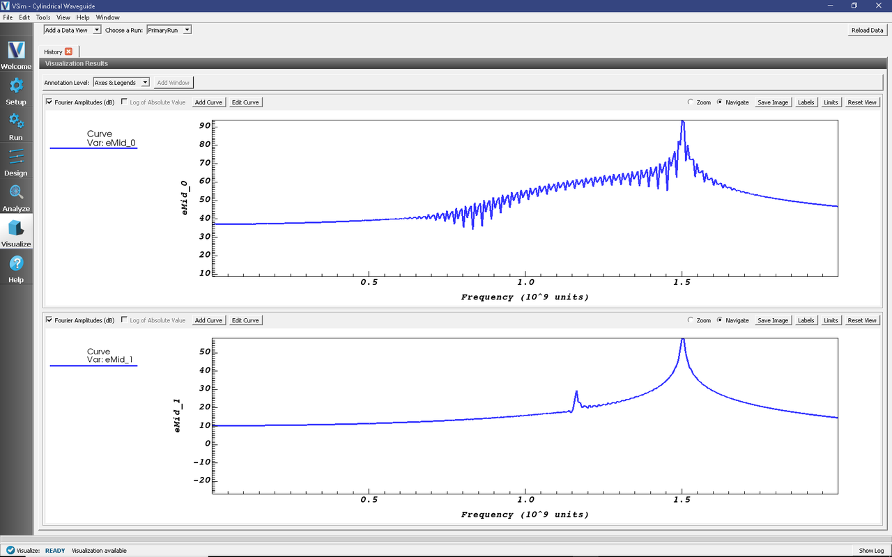
Fig. 355 Spectrum for the Cylindrical Waveguide example after the initial run.
One can see the TM mode in this spectrum. One can measure the mode frequency by projecting the spectrum down on the axis. With this simulation of 20,000 steps, for a total time of 103 ns, one expects the peak to have a width of roughly 1/103 ns or 0.01 GHz. This gives the error in the frequency from this method.
Computing More Accurate Modes
We can obtain more accurate frequencies using the Filter Diagonalization Method. To do this, we need to take a bit more data. We need to have the number of dumps equal to three times the number of modes, so we run again, restarting from dump 10 for another 300 steps, dumping every 50 time steps. This will give us an additional 6 dumps. The Run Window for this part of the simulation is shown in Fig. 356.
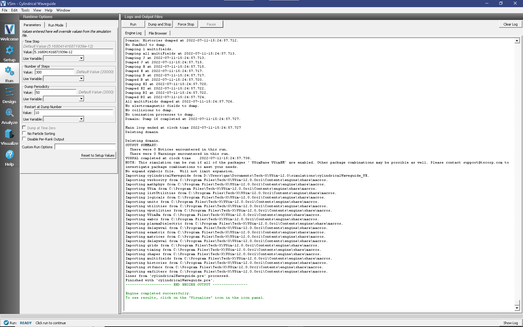
Fig. 356 Run Window for the Cylindrical Waveguide example for the second run.
We now move to the Analyze Window, open extractModes, and set the field to be
E. Then set the number of modes to be 2, and the begin and end dumps to be 10
and 16, respectively. Also set sampleType to 1. Upon hitting the Analyze
button in the upper right, one sees the analysis output as shown in
Fig. 357.
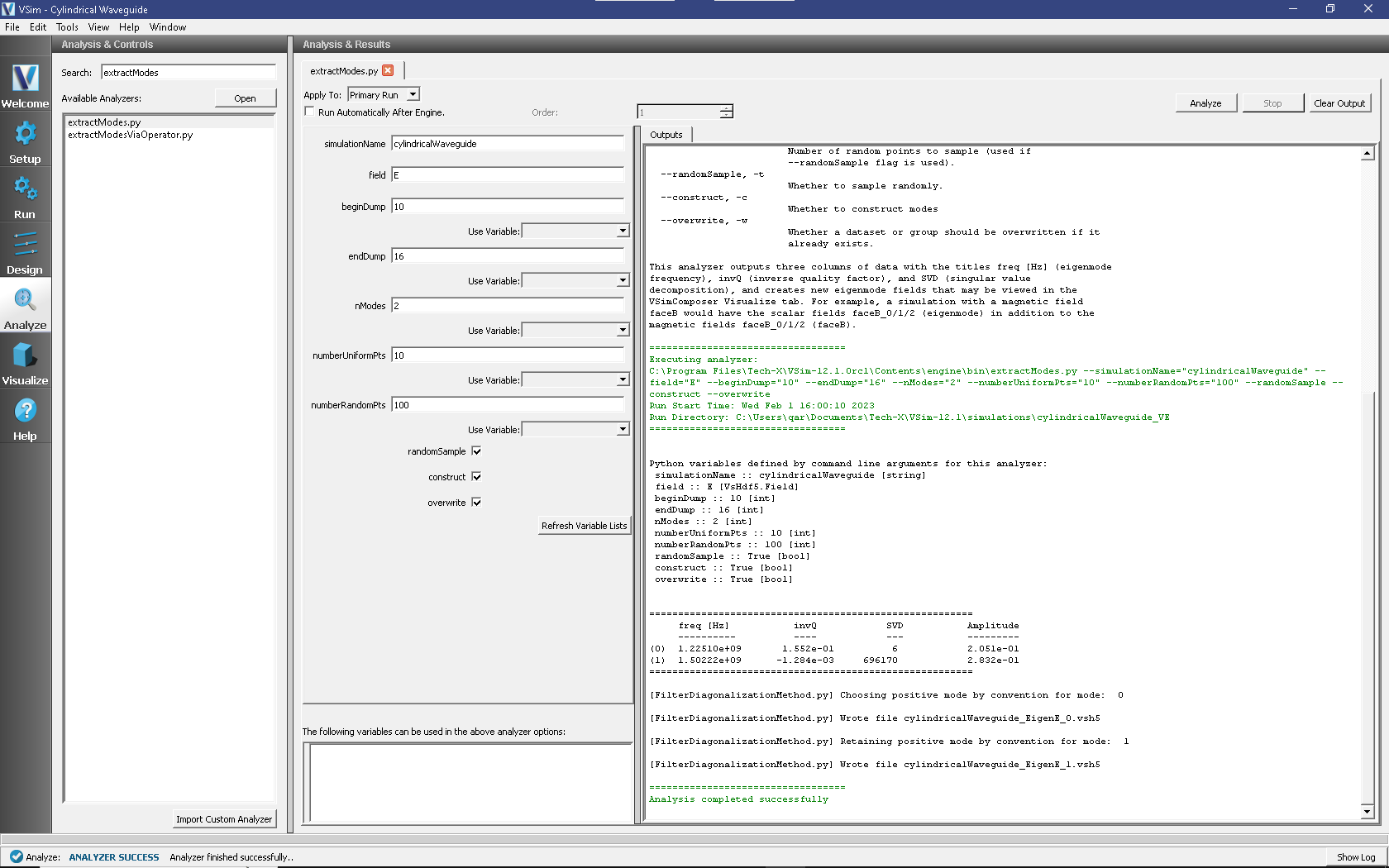
Fig. 357 Analysis window for the Cylindrical Waveguide example for mode extraction.
The computed mode frequencies are shown along with the inverse-Q values. Since this system is not lossy, the values of invQ, when significant, indicate that the mode calculations are dubious. However, we see that the 2nd mode has been well obtained.
These modes will now show up in the visualize panel, where one can reload the data, and modes will show up as seen in Fig. 358. The well obtained mode occupies dumps 1-16.
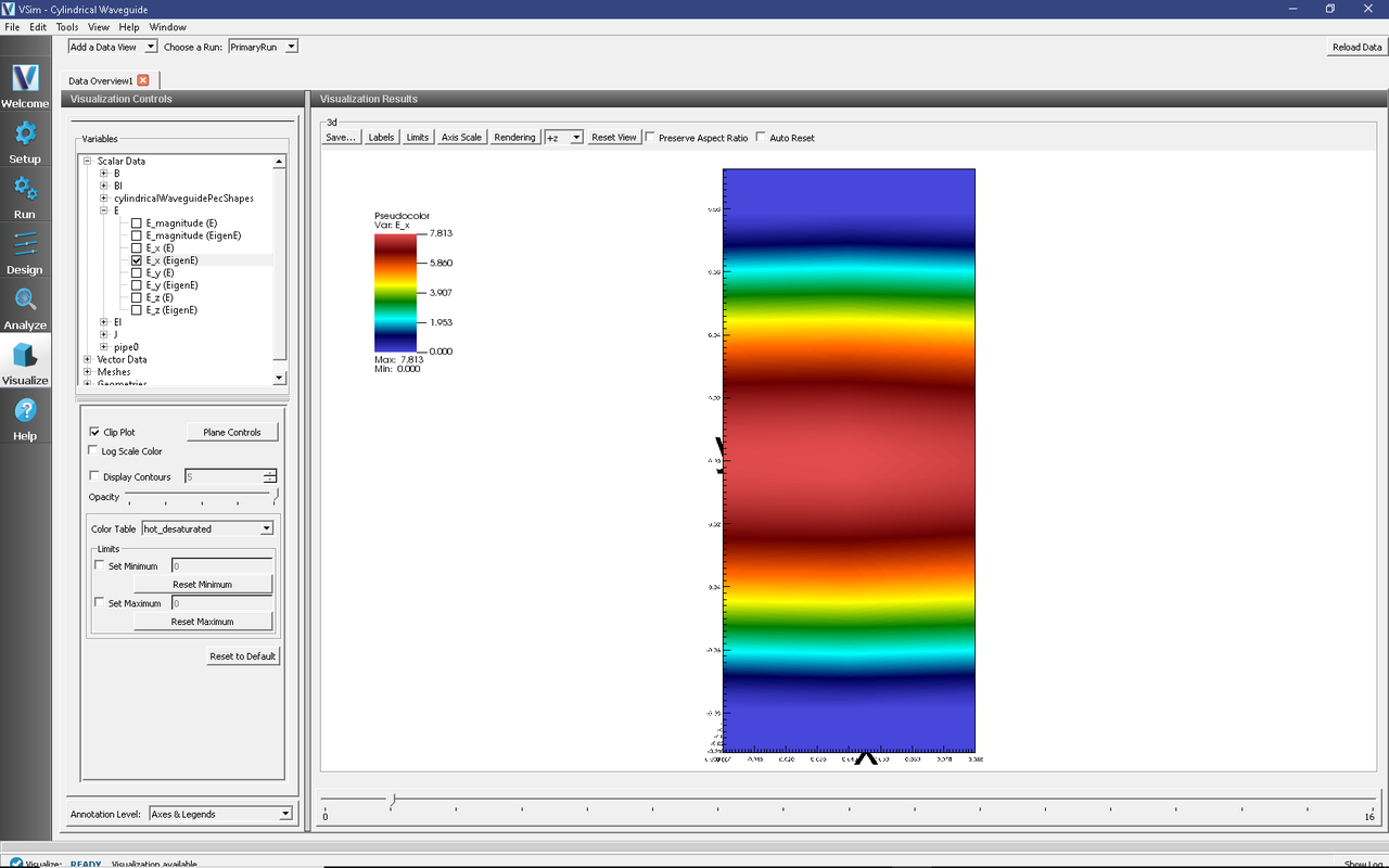
Fig. 358 Analysis window for the Cylindrical Waveguide example for mode extraction.