Electron Beam Driven Plasma Wakefield with Seperable Fields (eBeamDrivenPlasmawSeperableFieldsT.pre)
Keywords:
- electron driven, plasma wakefield, CLARA, PARS, AWAKE
Problem description
This example demonstrates a method to simulate an electron beam driven plasma wakefield accelerator. The electron beam initializes the field using a speed of light frame Poisson equation solve, then the fields and particles are evolved using FDTD EMPIC. We launch the electron beam from x=0 in the positive x direction using the Lorentz boosted Poisson fields to ensure that the simulation is self-consistent from start. The primary bunch generates a region of high field into which one might inject and accelerate a second bunch of charged particles. The example simulation uses parameters that are appropriate to the plasma acceleration research station (PARS) at the CLARA accelerator at Daresbury Laboratory in the UK.
Opening the Simulation
The Electron Beam Driven Plasma Wakefield example is accessed from within VSimComposer by the following actions:
Select the New → From Example… menu item in the File menu.
In the resulting Examples window expand the VSim for Plasma Acceleration option.
Expand the Beam Drive Acceleration (text-based setup) option.
Select Electron Beam Driven Plasma Wakefield (text-based setup) and press the Choose button.
In the resulting dialog, create a New Folder if desired, and press the Save button to create a copy of this example.
The basic variables of this problem should now be alterable via the text boxes in the left pane of the Setup Window, as shown in Fig. 470.
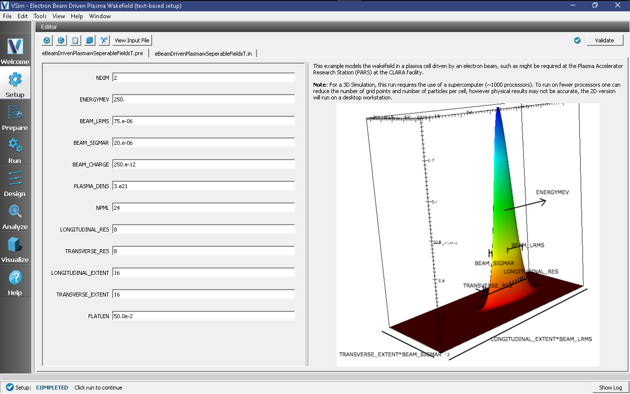
Fig. 470 Setup Window for the Electron Driven Plasma Wake example.
At this stage one can
choose parameters such as LONGITUDINAL_RES and TRANSVERSE_RES
which represent the longitudinal and transverse number of cells
per RMS bunch size. The minimum of 6 or default of 8, generates
a simulation that will complete reasonably quickly, but is not
adequate to generate good results. Consider 12 or 16 cells in
both dimensions to avoid a “checkerboard” pattern of numerical
noise from developing.
Input File Features
The simulation setup consists of an electromagnetic solver using the Yee algorithm and uses the initBeam macro to set up the initial beam properties. This takes the beam of variable weight particles and calculates self-consistent fields with which to initialize the simulation. As this beam travels near the speed of light, a moving window that co-propagates with the beam is employed. MALs are used on the transverse sides of the window to absorb outgoing waves. The plasma is represented by macro-particles, and both beam and plasma are moved using the Boris push. The particles in the plasma are variably weighted to represent the density ramp. It is assumed the plasma consists of pre-ionized heavy ions, which do not move in the time frame of the simulations.
One can specify the size of the region to be simulated through
LONGITUDINAL_EXTENT and TRANSVERSE_EXTENT, which
are measured relative to the longitudinal RMS size
BEAM_LRMS and transverse RMS size BEAM_SIGMAR of
the beam. The number of cells is determined by the settings of
LONGITUDINAL_RES and TRANSVERSE_RES, as shown in
the figure.
The plasma density is ramped up using a flat top cosine function,
by default, over a quarter of the longitudinal size of the
simulation window. This can be modified by viewing the input
file and editing the STARTRAMP and RAMPLEN
variables.
Running the Simulations
After performing the above actions, continue as follows:
Proceed to the Run Window by pressing the Run tab in the left column of buttons.
To run the file, click on the Run button in the upper left corner of the Logs and Output Files pane. You will see the output of the run in the right pane. This is shown in Fig. 471. The run has completed when you see the output, “Engine output has completed successfully.”
Running in 2D, you can expect a 2 core laptop to take a few minutes at the default resolution and run time.
To produce real significant results, a higher resolution is required by changing LONGITUDINAL_RES and TRANSVERSE_RES. Doing so will greatly increase the amount of time to run this simulation. It should also be run for longer than the default 3000 time steps.
The 3D simulation is about 100 times bigger, so 256 cores for a few hours is needed.
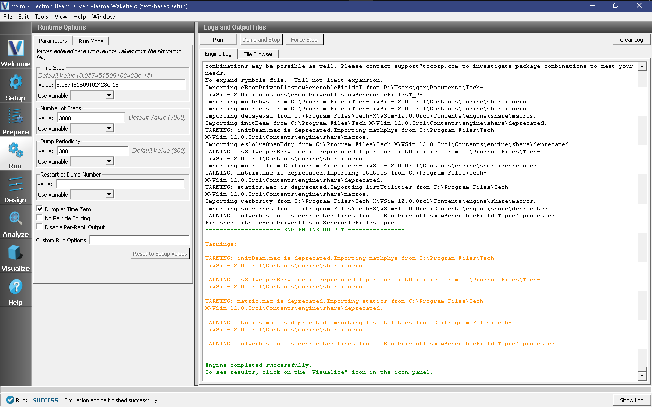
Fig. 471 The Run Window.
Visualizing the Output
After performing the above actions, continue as follows:
Proceed to the Visualize Window by pressing the Visualize tab in the left column of buttons.
View the electric field generated by the plasma as shown in Fig. 472 by doing the following:
Switch to Field Analysis in the Data View Controls pane
Set the Field to ElecFieldPlasma_x
Choose the Horizontal tab in Lineout Settings set the intercept to zero, and click Perform Lineout
Check the Auto Reset buttons on both the 2d and the Lineout plots. Sometimes it is necessary to expand the plot size in order for the box to appear. You can do this by pulling the divider between “Visualization Controls” and “Visualization Results” to the left and hiding it. Both the 2d and the Lineout plots should be larger now.
Move the dump slider forward in time.
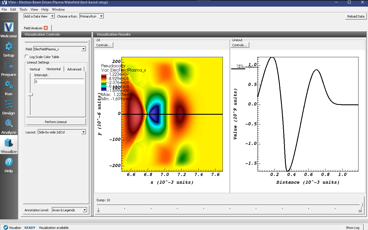
Fig. 472 Visualization of the longitudinal electric field as a color contour plot and longitudinal lineout.
The plasma density can be seen as shown in Fig. 473 by doing the following:
Switch to Data Overview in the Data View drop down
Expand Scalar Data
Select rhoPlasma
Click Auto Reset
Move slider all the way to the right.
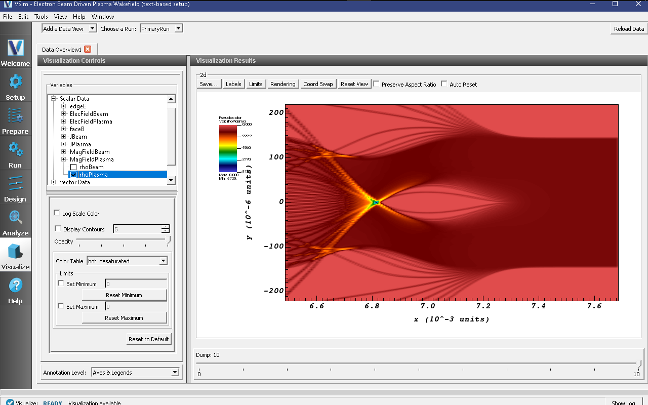
Fig. 473 Visualization of the longitudinal plasma density field as a color contour plot.