Visual-setup Simulations

After you open a new or example simulation that is not text-based, VSimComposer displays the Setup window containing an Editor pane with a Simulation Elements Tree, a Property Editor, and a Geometry View to allow for easy creation of your simulation. The icon panel remains available on the far left.

Note

A Navigation Pane can be shown by clicking and dragging on the vertical bar separating the Icon panel from the Editor pane. See Fig. 44.

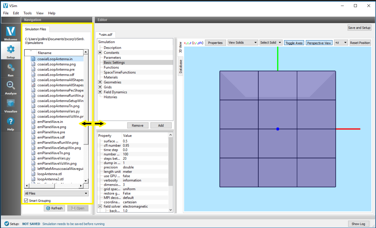
Fig. 44 The Navigation Pane

The following sections will go through each of the components of the Setup window.

For in depth information on each of the properties and possible values outlined or described in the rest of the chapter, please see VSim Reference: Visual Setup.

The figure Visual based setup window illustrates the layout of the VSimComposer Setup window using labels for the parts of the interface to which this introduction and the tutorials refer. See Fig. 45.

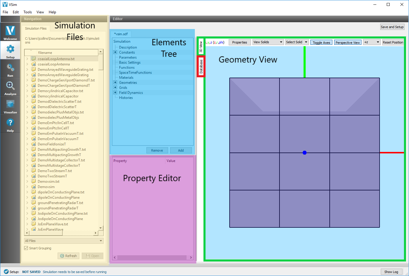
Fig. 45 Visual based setup window

Navigation Pane and Simulation Files

The Navigation pane contains a list of Simulation Files.

To enable convenient viewing of the list of simulation files, VSimComposer allows you to specify in what order as well as which type(s) of files you would like to view. Smart Grouping causes similar types of files to be displayed in the same area of the Simulation Files tab list. Turning off Smart Grouping causes files to be displayed in alphabetical order rather than by type. All Files indicates that you want to see all available files involved in the simulation. You could choose to limit your view to only Simulation Files, which are files such as input files and macros that can be edited in the VSimComposer Editor pane, or Text files, which include all types of human-readable file formats, or Data files, which include incremental dump files and output files that can be visualized.

Elements Tree Overview

You can navigate through the Elements Tree using either your mouse or your keyboard arrows. The up and down arrows will scroll up and down through the list of elements, while the right and left arrows will respectively expand and collapse the elements. To double click, press F2.

Highlighting a particular element in the tree will cause the Property Editor to update with Property/Value pairs that can be edited.

New elements can be added under an element in the tree by Right Clicking. This will be context sensitive, so for example right clicking Particle Sources will open up a tree of all types of available particle sources to choose from. Select one and click on it to add a new instance of that element.

Turn Off/On

This is an option available after Right Clicking or using the Add button. If it is selected it will gray out the element and it will not be translated into the input file.

This can be particularly useful for comparing results with and without a single element in place without having to go through the process of completely re-specifying it.

Create Clones

Any object can be right clicked and cloned, with all settings set the same as the object. Any number of copies can be created.

Buttons

• Undo

  This will Undo the last thing done. For example it will Undo the addition of an element, or the setting of a property.

• Add Multiple

  This is a shortcut that will add another instance of the last element added to the tree. Note that this can only be used on elements that are not visualized in the 3D view.

• Remove

  This will removed the highlighted element of the tree.

• Add

  This is the equivalent of right clicking a selected Element in the tree, and will present the same options.

We now discuss each of the sections of the Elements Tree.

Description

The Description element holds basic user-supplied text information about the simulation.

Constants

The Constants element contains a set of pre-defined physical constants that can be used in other elements of the simulation. You may also define your own by highlighting Constants and either clicking the Add button at the lower right of the Elements Tree or right-clicking and selecting Add Constant –> User Defined.

The name of the user-defined Constant can be modified by double clicking on the element in the Elements Tree and typing in a new name.

Note

A constant name can contain only alphanumeric characters and underscore and must start with a letter. Our convention is to use ALL_CAPS for constants.

A value can be given to the user defined Constant by double clicking on the value in the Property Editor. See Fig. 46.

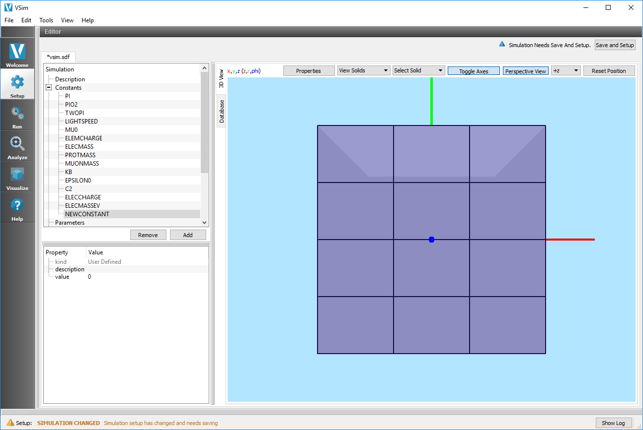
Fig. 46 Constant definitions

Parameters

The Parameters element is a location for evaluated, user-defined, variables that can be used in other elements of the simulation.

You can add a parameter by highlighting Parameters and either clicking the Add button at the lower right of the Elements Tree or right-clicking and selecting Add Parameter –> User Defined.

The name of the user-defined Parameter can be modified by double clicking on the element in the Elements Tree and typing in a new name.

Note

A parameter name can contain only alphanumeric characters and underscore and must start with a letter. Our convention is to use ALL_CAPS for parameters.

An expression can be given to the user defined Parameter by double clicking on the expression value in the Property Editor. You can use any of the Constants as well as any real number in the expression. See Fig. 47.

Note

If the expression is not valid, the parameter will appear in red in the Elements Tree.

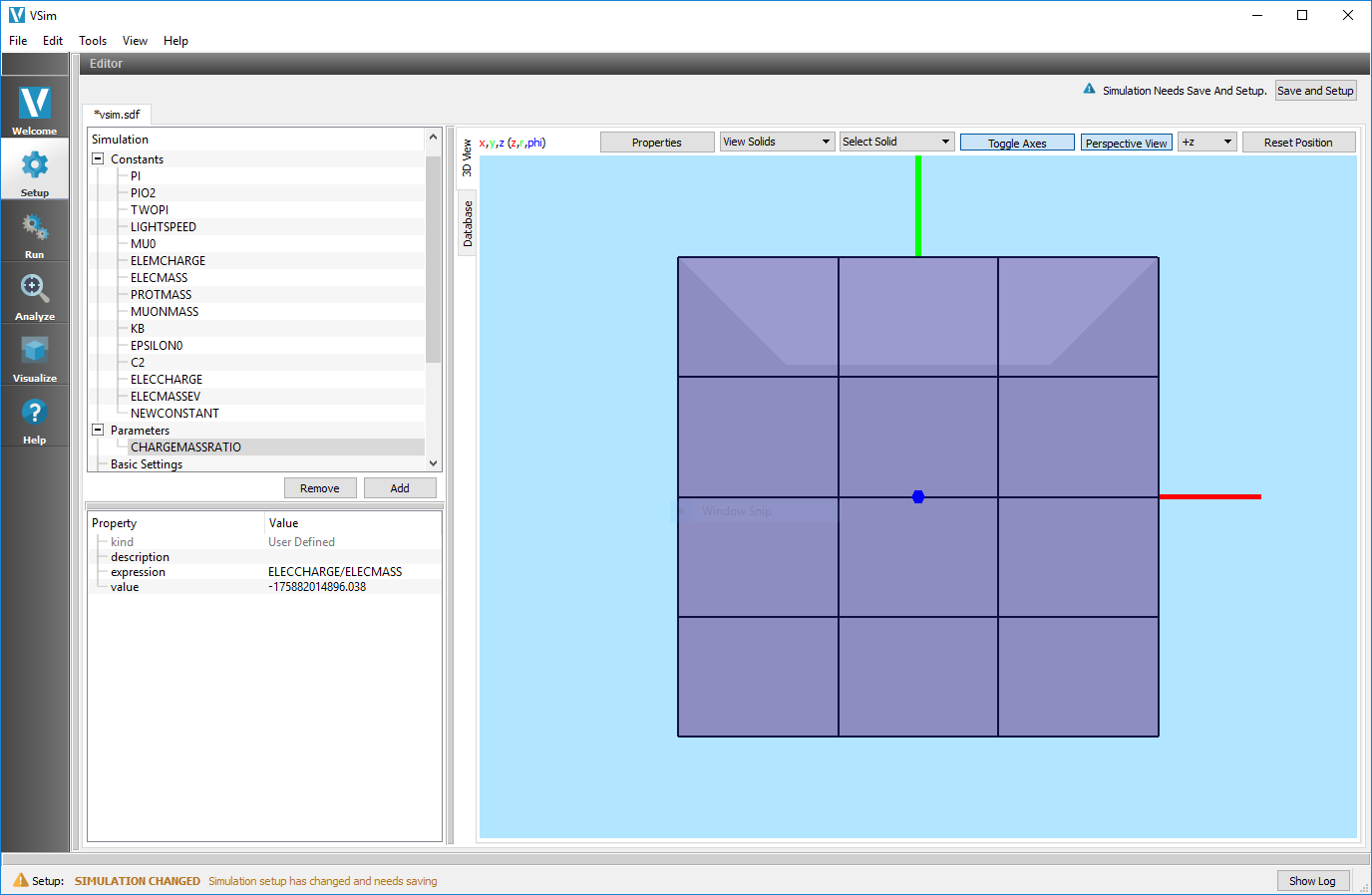
Fig. 47 Parameter definitions

Basic Settings

The Basic Settings element contains a group of property/value pairs that define the basic setup of the simulation.

Here you can find properties such as the type of field solve (electromagnetic, electrostatic, prescribed field, constant fields, hybrid fluid, or no field), the dimensionality (3D, 2D, 1D), whether or not to include kinetic particles in the simulation, and the time step.

Functions

The Functions element is a location for writing user-defined functions that can be used in simplifying the definition of a SpaceTimeFunction. The function can contain any number of arbitrary arguments and is not limited to the default values of x and y.

Note

A Function can be used to define another Function or a SpaceTimeFunction. Functions cannot be used to define an expression in other elements nor can they be used to define parameters. Expressions are defined by SpaceTimeFunctions.

To create your own function, highlight Function and either click the Add button at the lower right of the Elements Tree or right-click and select Add Function –> User Defined.

The name of the user-defined Function can be modified by double clicking on the element in the Elements Tree and typing in a new name.

Note

A function name can contain only alphanumeric characters and underscore and must start with a letter. Our convention is to use lowerCamelCase for function names.

You can define the Function by double clicking on the expression value in the Property Editor. You can use any of the Constants, Parameters, or Functions previously defined, as well as any real number or Python operator in the expression. See Fig. 48.

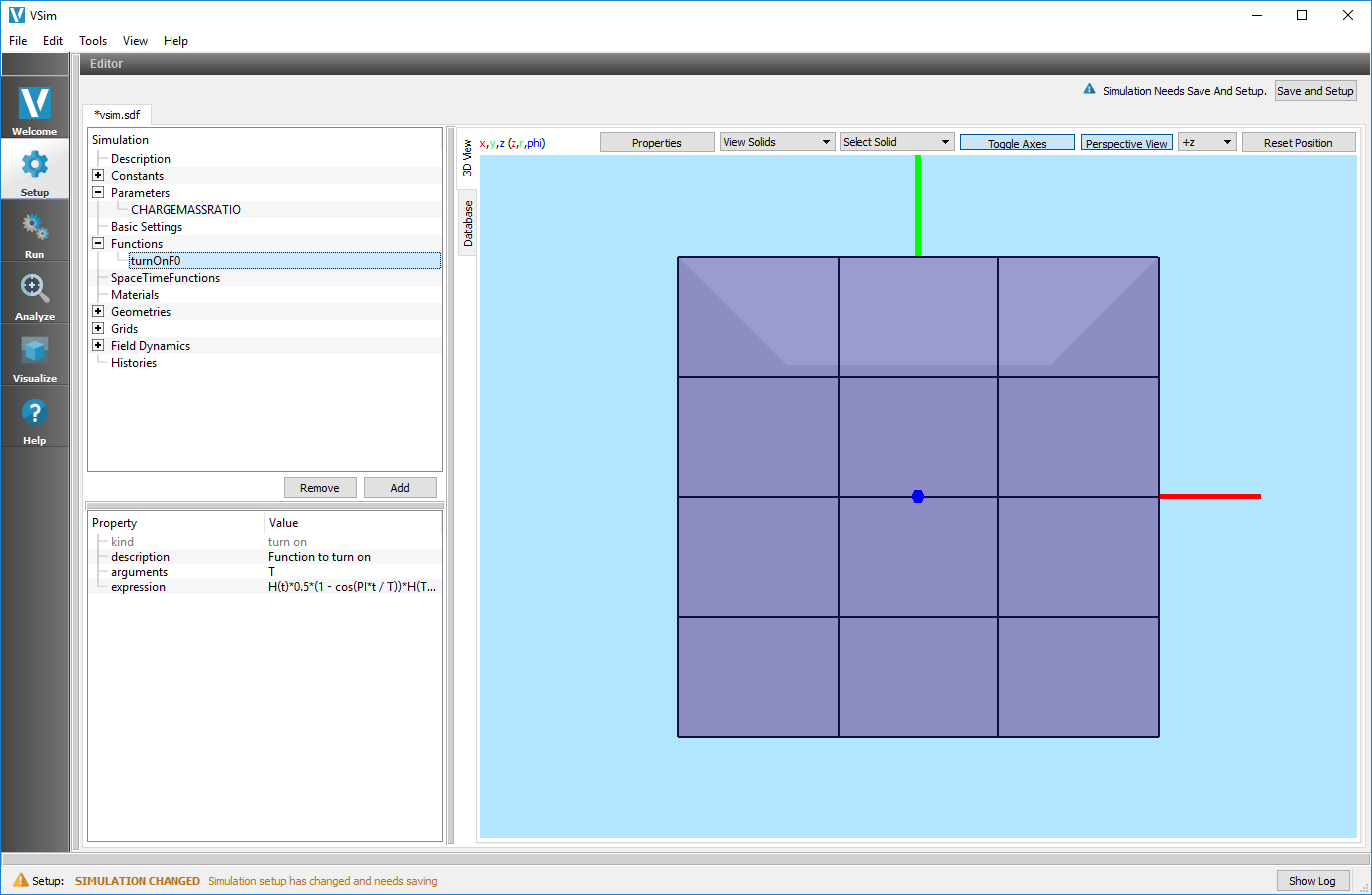
Fig. 48 Function definitions

SpaceTimeFunctions

The SpaceTimeFunctions element is a location for writing user-defined functions that specifically depend on the spatial and temporal variables x, y, z, and t. A SpaceTimeFunction can be used in other elements of the simulation by right clicking on the value and selecting the defined SpaceTimeFunction as shown in the figure SpaceTimeFunctions definitions.

To create your own function, highlight SpaceTimeFunction and either click the Add button at the lower right of the Elements Tree or right-click and select Add SpaceTimeFunction –> User Defined.

The name of the user-defined SpaceTimeFunction can be modified by double clicking on the element in the Elements Tree and typing in a new name.

Note

A SpaceTimeFunction name can contain only alphanumeric characters and underscore and must start with a letter. Our convention is to use lowerCamelCase for SpaceTimeFunction names.

You can define the SpaceTimeFunction by double clicking on the expression value in the Property Editor. You can use any of the Constants, Parameters, or Functions defined above, as well as any real number or Python operator in the expression. See Fig. 49.

Note

With SpaceTimeFunctions you may type in the name of a Constant or Parameter directly, however if you are to change the name of the Constant / Parameter used it will not automatically update to the new name, as it will in other elements of the SDF file.

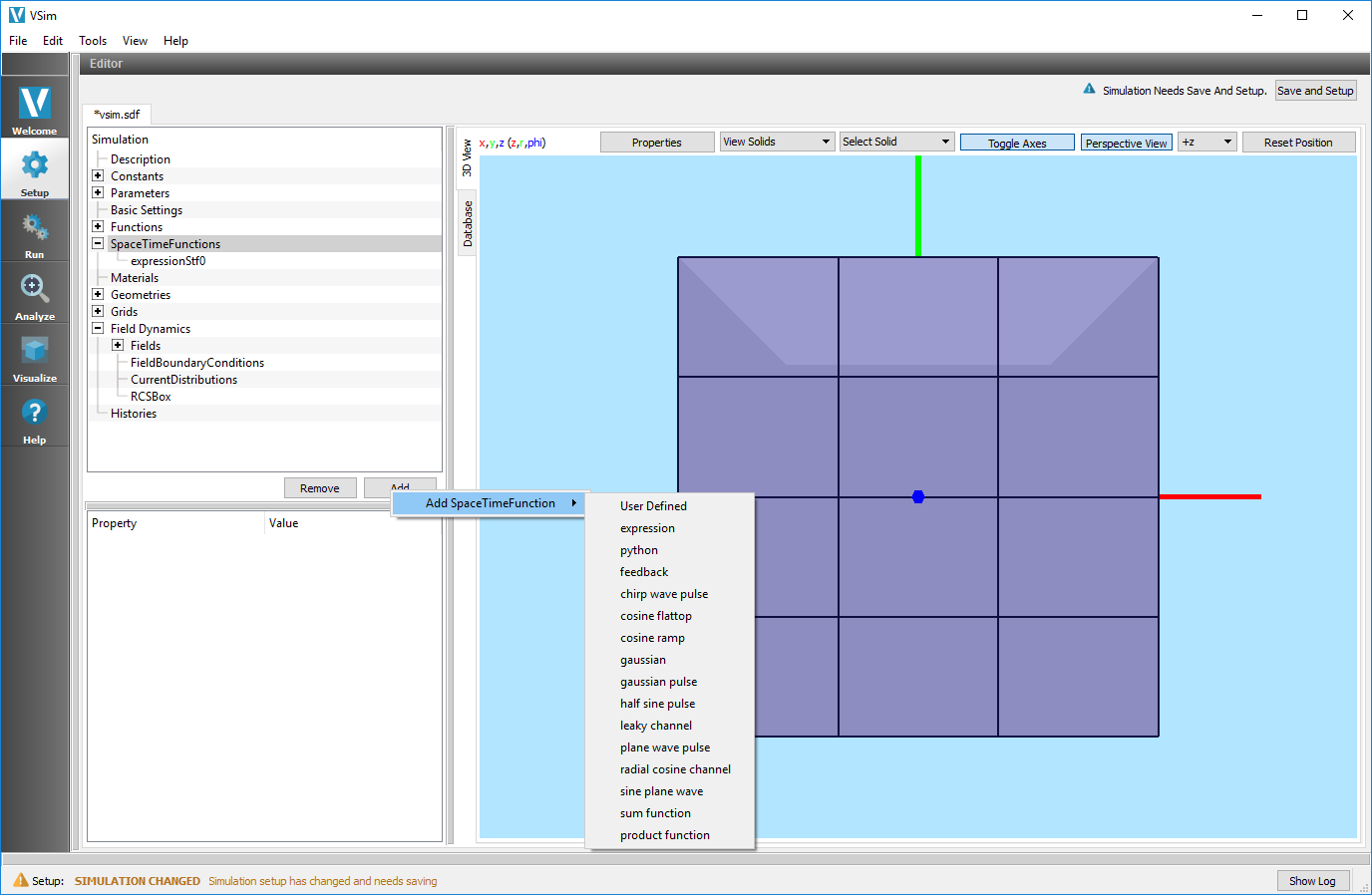
Fig. 49 SpaceTimeFunctions definitions

Materials

The Materials element holds information about any materials used in the simulation. There are some Materials built into VSim, and the user may import other desired materials.

To import a Material, either click the Add button at the lower right of the Elements Tree or right-click and select Import Materials.

The Materials file must have the extension .vmat. You can specify your own materials file to import special materials specific to your simulation. See Fig. 50.

Note

Tech-X has a standard materials file distributed with VSim. It is located in the data folder of your installation.

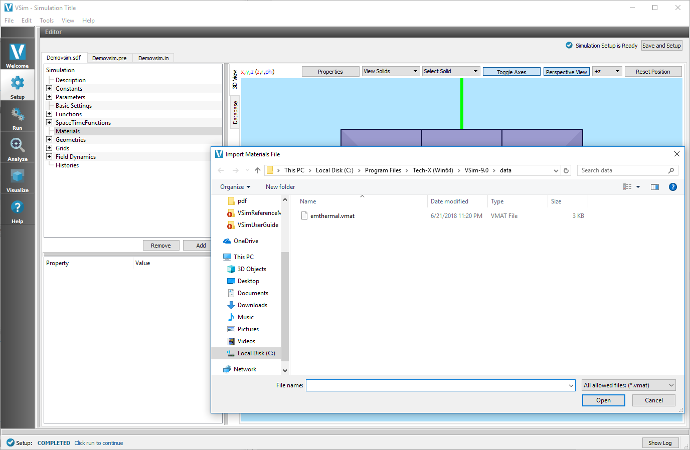
Fig. 50 Importing materials

Once a material file has been imported into VSimComposer, you can add a specific material to your simulation by highlighting the material of choice and clicking on the Add To Simulation button.

After a material is in the simulation, you can see it under the Materials element. The material properties can be modified, if desired. The Materials can be assigned to a geometry in the material property in the Properties Editor pane. See Fig. 51.

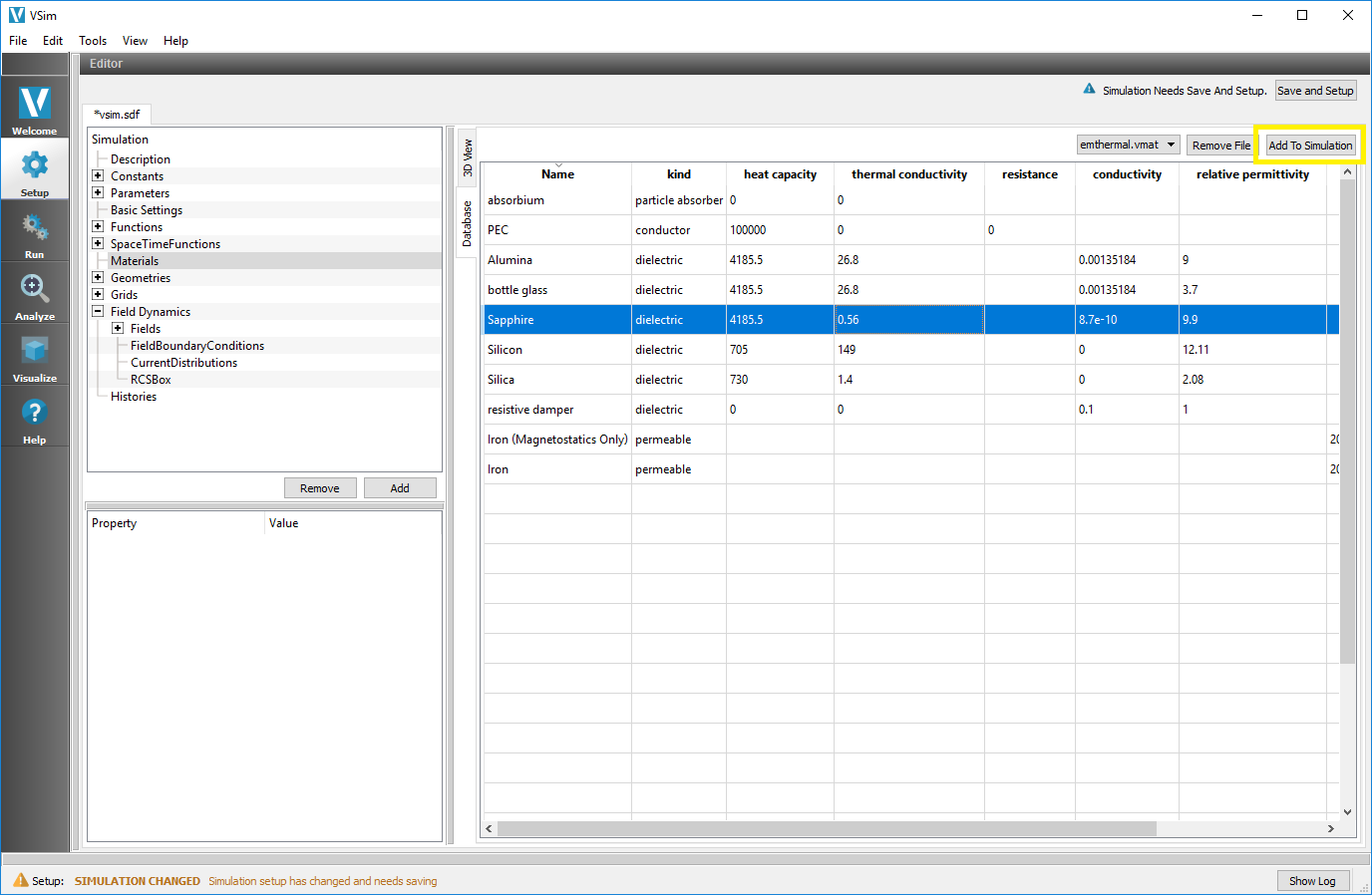
Fig. 51 Adding materials to the simulation.

Geometries

The Geometries element contains information about any geometries that are in the simulation. You can import a file, or create your own with CSG. Geometries present in the simulation can be modified, for example, healed, with holes closed.

Expanding the Geometries sub-elements view will show the individual parts (if any) of the imported geometry, or CSG built geometry.

To hide a specific part, uncheck the box next to it.

Note

Hiding a part of the geometry will not remove it from the simulation. VSim will use the full geometry defined in the imported file.

For use in the simulation, a Geometries part MUST have a material assigned to it, other wise it is ignored (treated as vacuum).

The material can be assigned to a geometry by double clicking on the material value in the Properties Editor. Note that the value of the dielectric assigned to the material, and hence the geometry, is only used if the field solve is electromagnetic. If you are using an electrostatic field solve, the dielectric must be assigned using SpaceTimeFunctions. Two examples illustrate the difference in how VSim handles dielectrics in the electromagnetic and electrostatic field solves: “Dielectric in Electromagnetics” and “Dielectric in Electrostatics” both of which are part of the “VSim for Electromagnetics” examples.

The color of geometry can be set in the Properties Editor after selecting the item line of that geometry in the tree. Not that selecting an item is different that selecting the visibility checkbox of that geometry item. Selecting the item means clicking on the line of the item anywhere but at checkbox. Once an geometry item is selected a color property line should appear in the Properties Editor. Double click on the color box in the Value column to bring up a Select Color dialog window to set the color. The transparency control is “alpha” on Windows and Linux (see Fig. 52) and “opacity” on Mac (see Fig. 53) can also be set in the Select Color dialog.

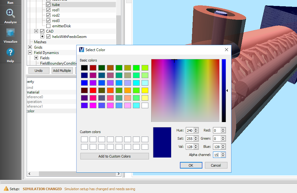
Fig. 52 Setting the color property of a geometry through the Select Color dialog on Windows and Linux. The alpha controls the transparency of the selected geometry.

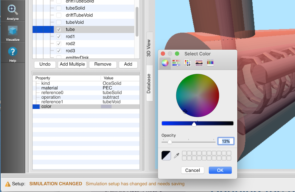
Fig. 53 Setting the color property of a geometry through the Select Color dialog on Mac. The opacity controls the transparency of the selected geometry.

Importing a Pre-defined Geometry

To import a geometry into your simuation, highlight the Geometries element in the Elements Tree and click on the Add –> Import Geometries button located at the bottom of the Elements Tree, or simply right click on the Geometries element –> Import Geometries.

Here you can navigate to a supported file type and open the file. Supported filed types include:

• Step Files (.stp, .step, .p12)

• STereoLithography Files (.stl)

• Visualization Toolkit Files (.vtk)

• Polygon File Format (.ply)

Building Your Own Geometry

You can build your own geometry using Constructive Solid Geometry (CSG) to create a complex shape by combining simple shapes using boolean operators.

To do this, highlight the CSG element and right click Add Primitive and select one of the pre-defined shapes. See Fig. 54.

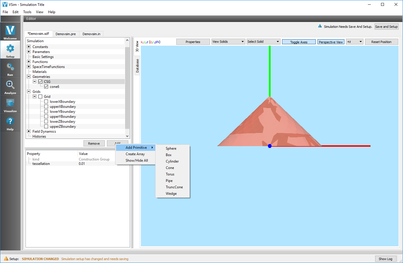
Fig. 54 Constructive Solid Geometry (CSG)

After multiple CSG shapes have been added, you can either subtract, union, or intersect them with a boolean operation. This will create a new Geometries element.

To do this, highlight the number of shapes you would like to include in the boolean operation, right click, and select the boolean operation you want. See Fig. 55. To highlight the second shape on Windows, hold down the ‘control’ button before selecting the second shape.

Note

The order of highlighting your shapes matters when doing the subtract boolean operation. The second shape will be subtracted from the first. The boolean operation menu will show the operation to be performed based on the order of highlighting.

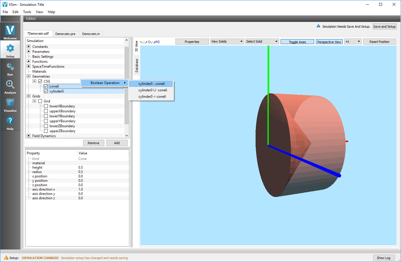
Fig. 55 Constructive Solid Geometry (CSG) Boolean Operator

Note

If a shape is not part of a combined shape through a boolean operation, you can assign a material to it. Once a shape has been combined with another shape, only the combined shape may be assigned a material.

Array Operations

Both CSG and CAD objects may be duplicated with array operations. To do this right click the object in question, and select Create Array. This will then open a dialog window to select the X Count, Y Count, and Z Count which will specify the number of objects to create in the respective axial direction. A drop down menu is also available to specify this number with a Constants or Parameter. X Spacing, Y Spacing and Z Spacing will control the spacing between objects - this spacing is in reference to the object in question. Similarly it is possible to assign a Constant or Parameter using the same drop down menu.

There is a Check box available to Union Created Shapes which will perform a union boolean operation between all shapes.

This dialog box is shown in the image below

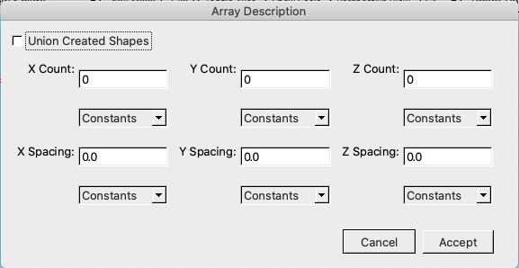
Fig. 56 Array Creation

Note

If using a constant or parameter, to define number of array elements/spacing it will hardcode to the value of that constant/parameter at the time of array creation. It will not update the number of elements/spacing should the value of that constant/parameter later change.

Creating Triangulated Surfaces

One can perform many other operations on surfaces in this interface, including analysis of geometries, which involves determining the number of separate surfaces that a geometry contains, and healing of geometries, which involves making them water-tight, closing up any holes. to triangulated form. One can also generate the simulation mesh for the geometries, and visualize it, which allows one to see whether the geometries have fidelity sufficient for a quality simulation.

Separating geometries

A common flaw is a CAD file that contains many objects, only some of which are required for the simulation. These objects may also interfere with one another, and may obstruct viewing angles. To begin, one imports the geometry to visually inspect it and see what it contains. One may then use the Separate Surfaces command to identify individual objects in the file and extract them into separate files for further use. This is invoked through the menu shown in Fig. 57, which comes up through a right click on the geometry.

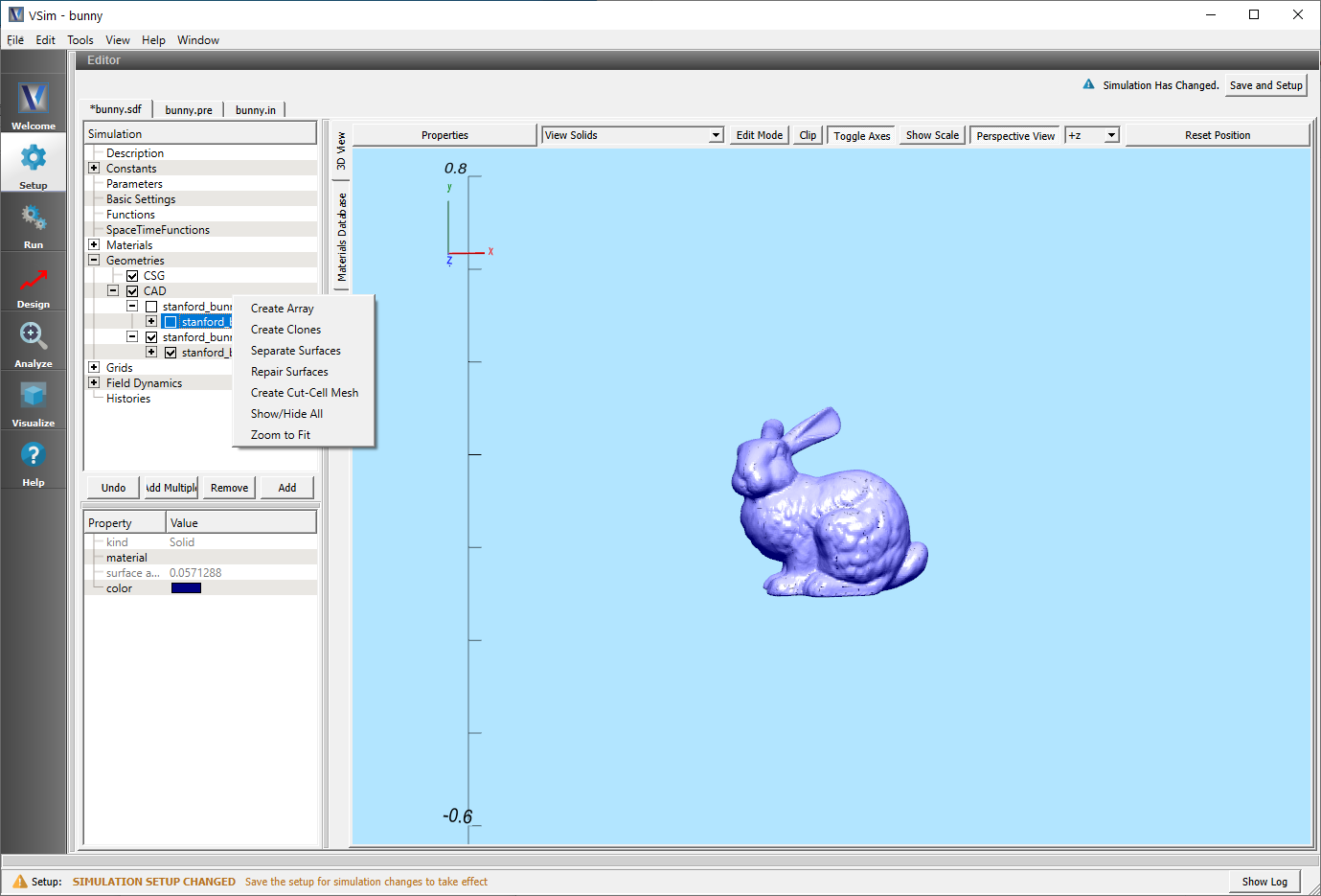
Fig. 57 Geometry analysis menu.

Selecting Separate Surfaces brings up the window shown in Fig. 58. Through this interface, one can separate the surfaces. Ultimately, one saves the surfaces for use as separate geometrical items in the simulation. Regardless of what options are chosen in this dialog, the original geometry object will not be changed.

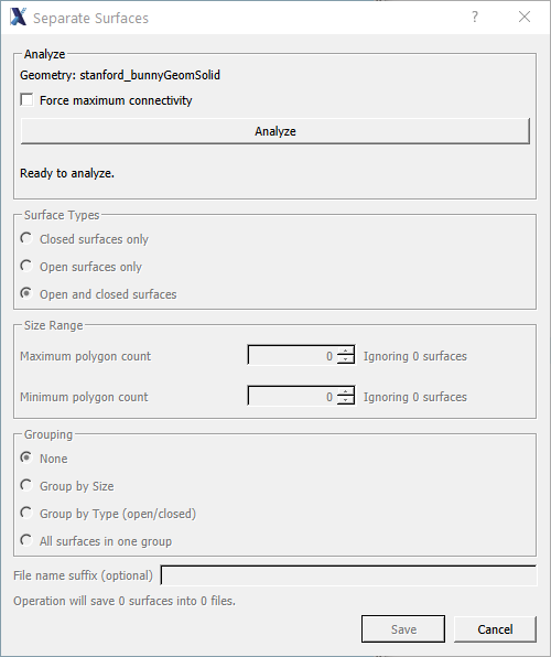
Fig. 58 Window for separating surfaces.

The first step is to “Analyze” the geometry, which will calculate the connectivity between each of the polygons that make up the geometry (triangles, quads, etc). By default, this step will not resolve any ambiguous connectivity - any polygon that could be a part of multiple geometries will be treated as a separate surface. To allow this step to attempt to resolve these ambiguities, one may turn on “Force maximum connectivity”. This step may take some time if the geometry is large or particularly complex.

The second step is to identify what types of surfaces to extract. One may choose to extract only closed surfaces, only open surfaces, or both. One may also set a size range for the extracted geometries. Only objects that satisfy all of the given conditions will be extracted.

The final step is to choose how the extracted surfaces will be saved. By default, each surface will be extracted into a new geometry object. You may also choose to group all geometries with the same size, or with the same type, or you may choose to save all surfaces into a single new geometry object. You may also supply an optional suffix to be appended to each of the extracted geometries. Upon being saved, the separate objects will show up in the Geometries tree.

For complex geometries, it may be desirable to use Separate Surfaces multiple times. For example, one may first choose to extract all geometries that are “open”, i.e. geometries that must be repaired before use. One may then choose to extract only the largest of these geometries, discarding any objects that consist of only one or two triangles. Finally, one may save each of these large geometries into separate files for further analysis and repair.

Healing geometries

Imported geometries may also have damage, such as holes, that will negatively affect the simulation. To detect and repair such geometry issues, one may use the Repair Surfaces command shown in Fig. 57. A dialog will appear that will guide you through the process. Again, regardless of what options are chosen in this dialog, the original geometry object will not be changed.

The first step is to “Analyze” the geometry, which will calculate the connectivity between each of the polygons that make up the geometry (triangles, quads, etc). By default, this step will not resolve any ambiguous connectivity - any polygon that could be a part of multiple geometries will be treated as a separate surface. To allow this step to attempt to resolve these ambiguities, one may turn on “Force maximum connectivity”. This step may take some time if the geometry is large or particularly complex.

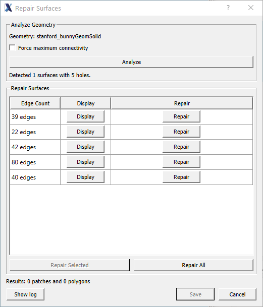
Fig. 59 Window for repair surfaces.

When analysis has completed, the dialog will display a list of all holes (if any) in the target geometry. The “Edge Count” value is the number of edges that border the hole. A hole with three edges is a triangle, four edges is a quad, and more edges that that is a larger polygon. The “Display” button will rotate and zoom the view in an attempt to present the given hole to the camera. Note that this may not be successful if the hole is topologically complex or hidden by another surface. The “Repair” button allows you to fill the hole with new triangles. You may then also undo the operation if the repair is unsatisfactory. Upon conclusion of Repair, the patch needed for the repair shows up in the tree.

Composer includes several different healing algorithms. By default, the choice of algorithm is performed automatically depending on the characteristics of each hole. However, one may override the automatic choice if the resulting patches are not acceptable.

To finalize the process, press the “Save” button. Another dialog will appear that will allow you to choose how to save the results. “Export Healed Geometry” will create a new geometry object that includes the original geometry and any newly generated triangles. “Export Patch” will create a new geometry object that contains only the newly generated triangles. The healed object will then show up in the tree for use in the simulation.

Generating Simulation (Cut-Cell) Meshes

Once a shape has been created using a primitive or imported, the shape will appear under the “CSG” tab if you created the shape or “CAD” tab if you imported the shape. If you want to view the mesh that is used to represent that shape in the simulation, then right click on the shape and click on Create Cut-Cell Mesh. The mesh will be added under the “Meshes” tab in the Visualization pane.. If you uncheck the box next to the shape under the “Geometries” tab, this will hide the solid shape, revealing the surface meshing used in the simulation. If the mesh is not revealed, check the box next to the shape under the “Meshes” tab. The resolution of the surface mesh depends on the resolution of the grid, which is determined under the “Grids” tab. Increasing “xCells” makes both the grid and surface mesh finer in the x-direction.

Grids

The type of grid is determined in the Basic Settings element. Its parameters are determined in the Grid element.

By default, a uniform Cartesian grid is added to your simulation with dimensions of 1m x 1m x 1m and cell numbers of 3, 4, and 5 in x, y, and z respectively.

To modify the type of grid, change the Basic Settings properties coordinate system, dimensionality, and grid spacing. See Fig. 60.

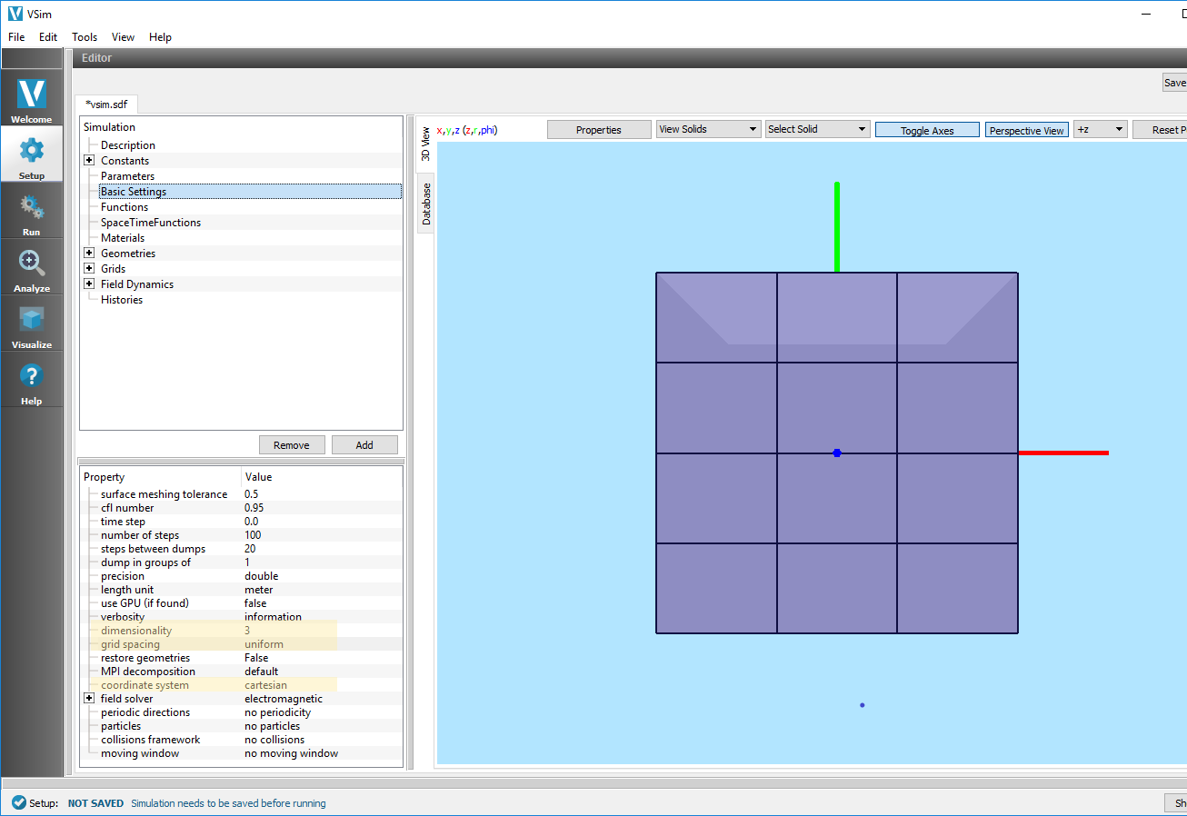
Fig. 60 Grid choices

The size of the domain can be set using the Min and Max properties of a uniform Grid element or with the minimum and maximum values of the SectionBreaks properties of a variable Grid element. The number of cells in each direction can also be specified. See Fig. 61.

Note

Only one grid may be added to any one simulation at a time.

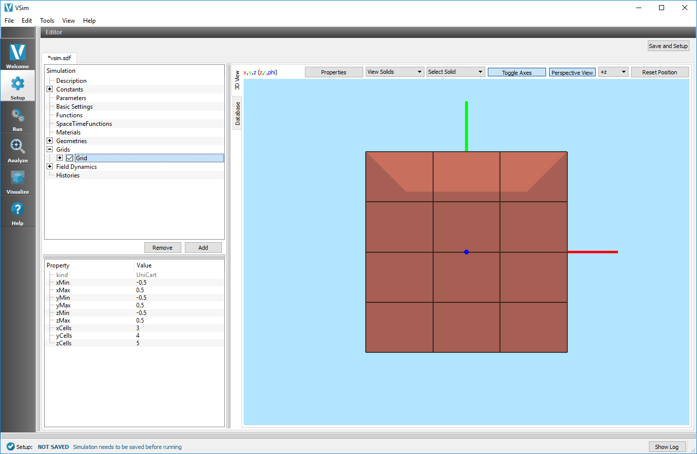
Fig. 61 Grid settings

Note

A grid can be resized to fit the bounds of a geometry by right clicking on the Grid element and choosing Resize Grid. Resizing the grid puts in numbers, replacing any constants and parameters.

Field Dynamics

The type of field solver is determined in the Basic Settings element. Its parameters are specified in the Field Dynamics element.

Field Solver

4 field solvers are available in VSim

Electromagnetic Solver

The electromagnetic solver will solve the E, B and if explicitly included (or particles are in the simulation) a J field is added to the simulation.

Electrostatic Solver

The electrostatic solver will solve an E, Phi and Charge Density, with the option to include external magnetic fields.

Prescribed Fields Solver

The prescribed field solver can be used to import previously solved external fields, and then provide a time dependent variation. This can be used when studying particle dynamics, particularly in multipacting simulations.

Constant Fields Solver

The constant field solver can be used to apply a constant field in particle simulations. Particle movement will not impact these fields, however the field will impact particle movement.

No Field Solver

A no field solver is used if only Particle Dynamics are to be studied, without the impact of fields.

Hybrid Fluid Solver

The hybrid fluid solver enables hybrid fluids, which cannot interact with standard field solves.

Fields

Depending on the type of solver chosen, default fields will be initialized in the simulation. For an electrostatic simulation, default fields will be Phi, Charge Density and Electric Field. You can optionally add a Background Charge Density field or External Field by clicking the Add –> Add Field button located at the bottom of the Elements Tree, or simply right clicking on the Fields element –> Add Field.

An External Field is used for importing a Magnetic field in electrostatic simulations with particles.

For an electromagetic simulation, default fields will be Electric Field and Magnetic Field. You can optionally add a Current Density field or External Field by clicking the Add –> Add Field button located at the bottom of the Elements Tree, or simply right clicking on the Fields element –> Add Field.

An External Field in electromagetic simulations can be a Magnetic, Electric, or Current field. External fields are used to effect particle movements in simulations.

Field Initial Conditions

An initial condition can be added to any field by clicking the Add –> Add FieldInitialCondition button located at the bottom of the Elements Tree, or simply right clicking on the particular Field element –> Add FieldInitialCondition. See Fig. 62.

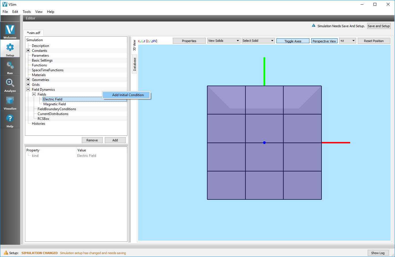
Fig. 62 Adding an initial condition to a field

Field Boundary Conditions

A boundary condition can be added to any field by clicking the Add –> Add FieldBoundaryCondition button located at the bottom of the Elements Tree, or simply right clicking on the particular Field element –> Add FieldBoundaryCondition.

Current Distributions

A current distribution can be added to any field by clicking the Add –> Add CurrentDistribution button located at the bottom of the Elements Tree, or simply right clicking on the particular Field element –> Add CurrentDistribution.

A distributedCurrent is a volume current source where you can provide the min and max values in each direction. A distributedCurrent will show up on the Geometry View. You can hide a distributedCurrent by unchecking the box next to it. Hiding a current will not remove it from the simulation, it’ll just hide it from the geometry view. See Fig. 63.

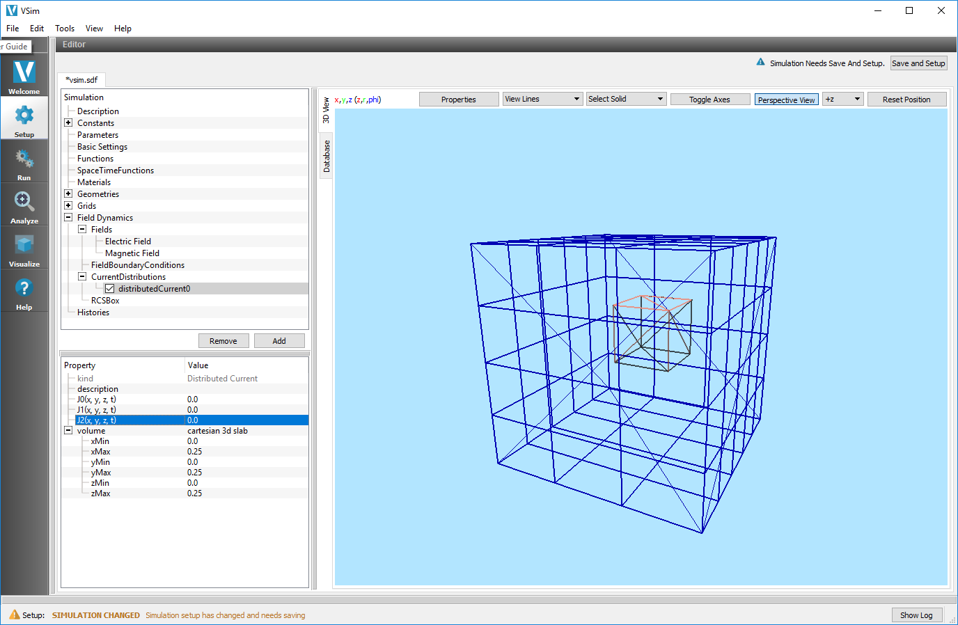
Fig. 63 A volume of current is shown in the smaller/interior box. The outer box is the grid.

Poisson Solver

The type of Poisson solve and any preconditioner can be set under the solver and preconditioner properties of the Properties Editor.

Note

Changing the solver type may introduce more properties due to the context-sensitive nature of the input.

Particle Dynamics

The inclusion of Particle Dynamics is determined by the value of particles in the Basic Settings element. If particles is set to no particles, then no particles are in the simulation and the Particle Dynamics element is hidden.

If particles is set to include particles then the Particle Dynamics element is shown and futher properties can be set.

The Particle Dynamics element holds information on any kinetic particles, background gases, and collisions in the simulation.

KineticParticles

Electrons, charged particles, and neutral particles can be added to the KineticParticles element.

To add kinetic particles, click the Add –> KineticParticle button located at the bottom of the Elements Tree, or simply right click on the KineticParticles element and select Add KineticParticle and then choose the type of particle you want to include.

The properties of each kind of KineticParticle are modifiable in the Properties Editor pane.

Fluids

Neutral Fluids can be added to the simulation. To add a fluid, right click the Fluids button and select Add Fluid

A fluid is a volume distribution where you can provide the min and max values in each direction. A fluid will show up on the 3D View. You can hide a fluid by unchecking the box next to it. Hiding a fluid will not remove it from the simulation, just hide it in the 3D view. See Fig. 64.

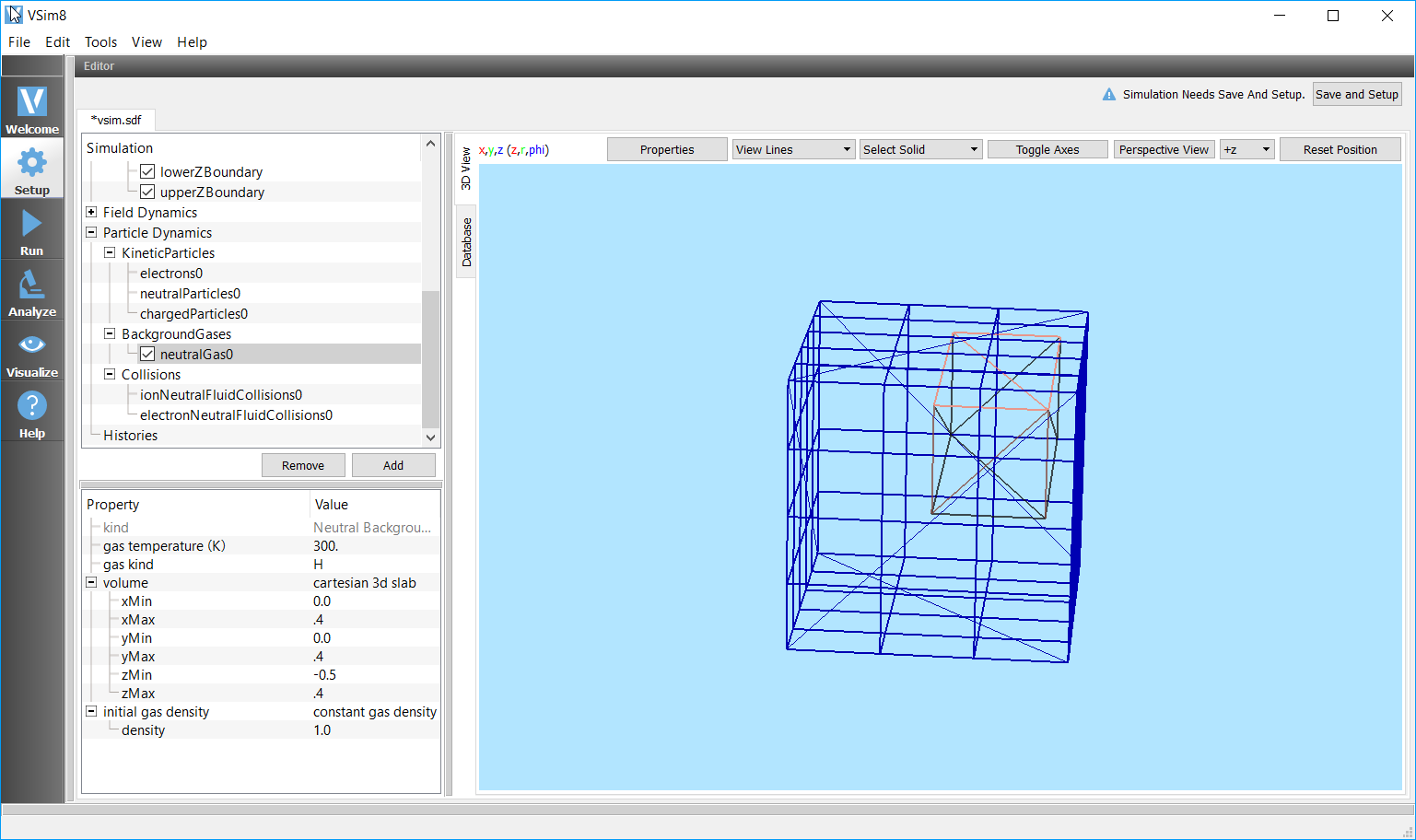
Fig. 64 A volume of fluid is shown in the smaller/interior box. The outer box is the grid.

Collisions

There are three frameworks for setting up particle collisions available in VSim. The newest, most flexible, and fastest is the Reactions framework. The Reactions framework supplants the Monte Carlo Interactions framework. The Impact Collider (called “ReducedCollisions” in the Visual Setup) framework is the oldest framework, and is limited to interactions between kinetic particles with a neutral fluid, but runs very quickly.

In the Visual Setup, only one framework can be used at a time.

Reactions

To include Reactions in the Visual Setup, first select the Basic Settings element of the setup tree and ensure that the particles dropdown menu is set to “include particles” and the collisions framework dropdown is set to “reactions.”

With these settings selected, collisions can now be set up within the Particle Dynamics element of the setup tree. The Reactions are organized between five options: Particle Particle Collisions, Particle Fluid Collisions, Three Body Reactions, Field Ionization Processes, and Decay Processes. By highlighting one of these five options, right clicking, and adding a collision process a user is setting a RxnProductGenerator`(see :ref:`VSim Reference Manual: Text Setup: Reactions <rxn-rxnProductGenerator> for more information on RxnProductGenerators).

Note

The distinction between the Particle Particle Collisions and Particle Fluid Collisions is artificial in the visual setup and is made for the convenience of the user.

After adding a collision process to the tree, the user then selects the reacting species, cross-sections/reaction rates, and other reaction attributes. The species and fluids in the drop down menu for reactants and products are limited such that only selections appropriate for the process are available. Charge and mass conservation is checked during the translation from .sdf to .in. If there is a charge or mass violation, an error will be thrown.

If the drop-down menu used to set the interacting particle species is empty, make sure you’ve added the necessary KineticParticle or BackgroundGas for the type of collision.

Reduced Collisions (Impact Collider)

To include Reduced Collisions in the Visual Setup, first select the Basic Settings element of the setup tree and ensure that the particles dropdown menu is set to “include particles” and the collisions framework dropdown is set to “reduced”. With these settings selected, collisions can now be set up within the Particle Dynamics element of the setup tree.

To add collisions between kinetic particles and a neutral background gas (fluid), click the Add –> Add ParticleFluidCollision button located at the bottom of the Elements Tree, or simply right click on the Collisions element and select Add ParticleFluidCollision and choose whether either Electron Neutral Fluid Collision or Ion Neutral Fluid Collision. After making a selection, a new element will appear in the tree. Choose the particle species and the background gas that will interact.

To add a specific collision process, highlight this new element and choose a specific collision process from the Add CollisionProcess menu which will appear next to the mouse arrow. When a specific collision process is added, a new element will appear. The cross-sections for the interaction process will be set in this element.

See Fig. 65 for an example of adding collisions to a simulation in the Visual Setup.

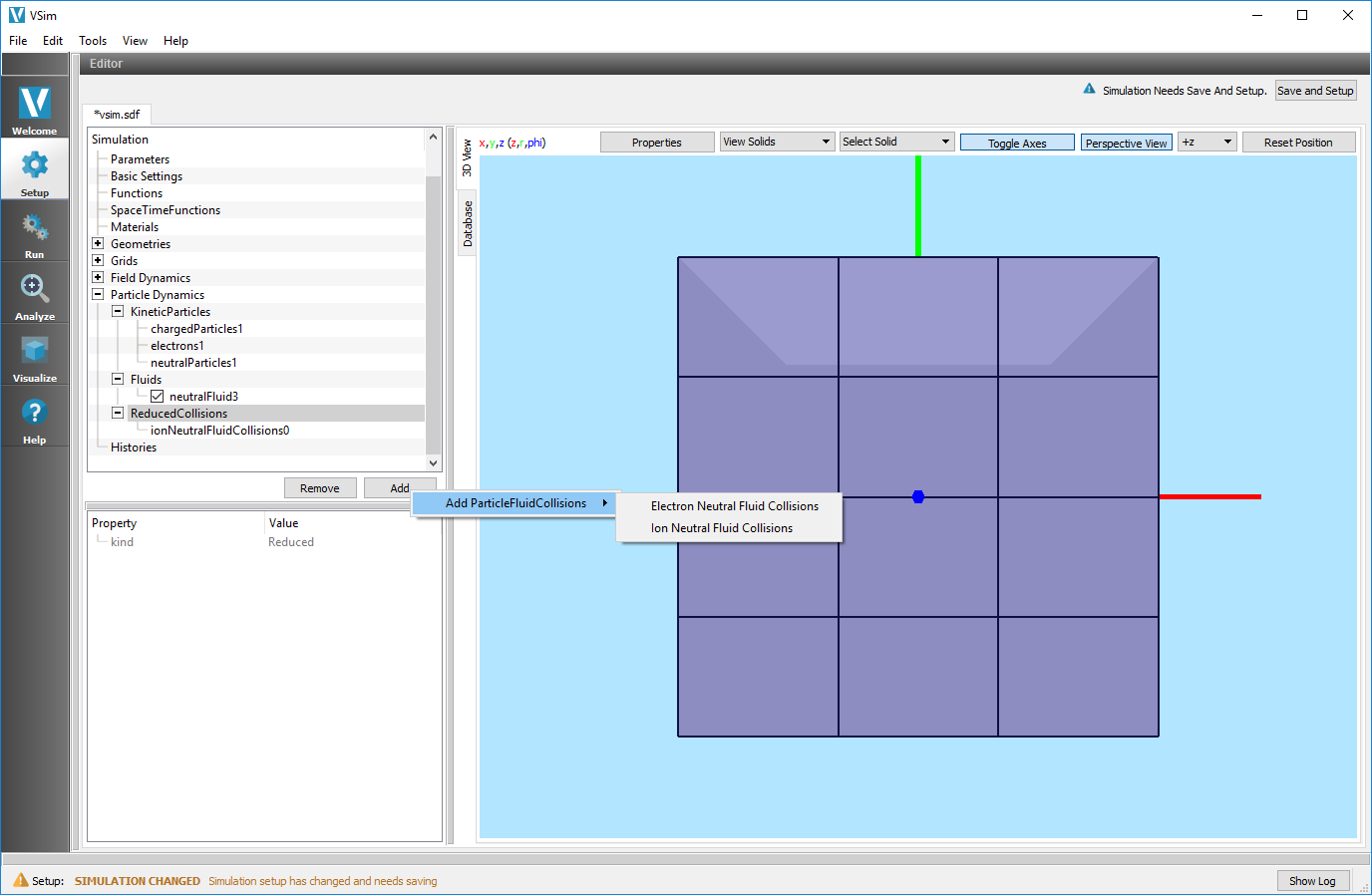
Fig. 65 Collisions

Monte Carlo Interactions

To include Monte Carlo Interactions in the Visual Setup, first select the Basic Settings element of the setup tree and ensure that the particles dropdown menu is set to “include particles” and the collisions framework dropdown is set to “monte carlo”.

With these settings selected, collisions can now be set up within the Particle Dynamics element of the setup tree. The Monte Carlo are organized between five options: Particle Particle Collisions, Particle Fluid Collisions, Three Body Reactions, Field Ionization Processes, and Decay Processes. The user can add a specific interaction process by highlighting one of these five options, right clicking, and selecting a process from the Add CollisionType menu.

After adding a collision process to the tree, the user then selects the reacting species, cross-sections/reaction rates, and other reaction attributes.

Histories

Histories are used to calculate and record data about fields and particles in a simulation.

ArrayHistory

An Array History will output an array of data for each time-step.

Possible Array Histories include:

• Far-Field Box Data

• Field Slab Data

• Particle Momentum

ComboHistory

Combo Histories are used to do operations on other histories. The operation is done at every time step and the resulting values are recorded as a new history. The output will be a 1D array of the value vs time.

Possible Combo Histories include:

• Binary Combination History

FieldHistory

Field Histories record on a per time-step basis. Field histories are used to measure quantities such as the value or energy of the field at a location. The output will be a 1D array of the value vs time.

Possible Field Histories include:

• Accelerating Voltage

• Electric Field Energy

• EM Field Energy

• EM Field on Plane

• Magnetic Field Energy

• Field at Position

• Poynting Flux

• Pseudo-potential

LogHistory

A Log History will record data on a per-event basis rather than at each time step. For instance, an Absorbed Particle Log will record information about each and every particle that strikes a chosen absorbing surface. The output will be a 1D array of the value.

Possible Log Histories include:

• Absorbed Particle Log

• Emitted Particle Log

ParticleHistory

Particle Histories record on a per time-step basis. Particle histories are used to measure quantities such as the total number of particles in a simulation at each step, or the current absorbed at a chosen absorbing surface at each step. The output will be a 1D array of the value vs time.

Possible Particle Histories include:

• Absorbed Particle Current

• Absorbed Particle Energy

• Emitted Current

• Number of Macroparticles

• Number of Physical Particles

• Particle Energy

• Particle Energy Change from Boundary

ComboHistory

A combo history is used to combine other histories, two types are available:

• Combination History

• Time Average

Property Editor

The Property Editor allows for setting of specific properties under each of the Elements from the Elements Tree for the simulation. Such properties might include sizes in the X, Y, and Z directions, the type of particles, and specifics of a field solve.

The Property and Value inputs are context-sensitive. The availability of a particular property may depend on other properties or selections of the Element Tree. For instance, changing the solver value in the PoissonSolver element will bring up a new set of solver properties to be set. Refer to the figure Constructive Solid Geometry (CSG) Boolean Operator (Fig. 55) to see the same principle with regard to geometry options.

Geometry View

The 3D View section can be used to view the simulation setup including the geometry, grid, and source.

Buttons

• Properties

  This will open a dialog that will allow edting the properties of the 3D View. Following changes can be made through this dialog: Set line width and point size. Choose how Colors will be assigned to shapes in the 3D View. See Fig. 52 for further information Set shininess of a shapes. Show or hide axes Show the coordinates of a clicked point of a geometry.

• View Solids

  This will show all objects as solid, can also be set to View Solids/Lines, View Lines (wireframe) or View Points

• Distance This will allow measuring distance between two points of a geometry. The clicked points and the distance will be visible at the bottom of the 3D View.

• Clip

  This will open up a drop down menu to clip the simulation view, with a chosen normal direction and coordinate to place the clip at.

• Toggle Axes

  A toggle button to show or hide the axes.

• Show Scale

  This will allow changing the scale shown be default, from nanometers to kilometers. Note that all values will remain in meters or as defined by the user, this is just used to rapidly change the scale shown in the setup menu.

• Perspective View

  This will reset to a perspective view for the 3D view.

• Axis Drop-down Menu

  Drop-down menu for choosing the axis from which the object is viewed.

• Reset Position

  Pressing this button will reset the camera view to be along the axis selected in the drop-down menu.

• Edit Mode

  Edit mode will allow application of transformations to a selected portion of a geometry. Here is the workflow: After switching to edit mode, click on “Add Volume Selector” to add a selector, then move the selector to desired location to overlap the geometry by changing its position through the property editor. After that, select the geometry node that is to be edited and click on “Perform Selection”. A new node will be added in the tree with the selected part being red in color. All the transformations that are applied to this new node only gets applied to the red portion of the geometry. Click on “Done Editing” to exit this mode.

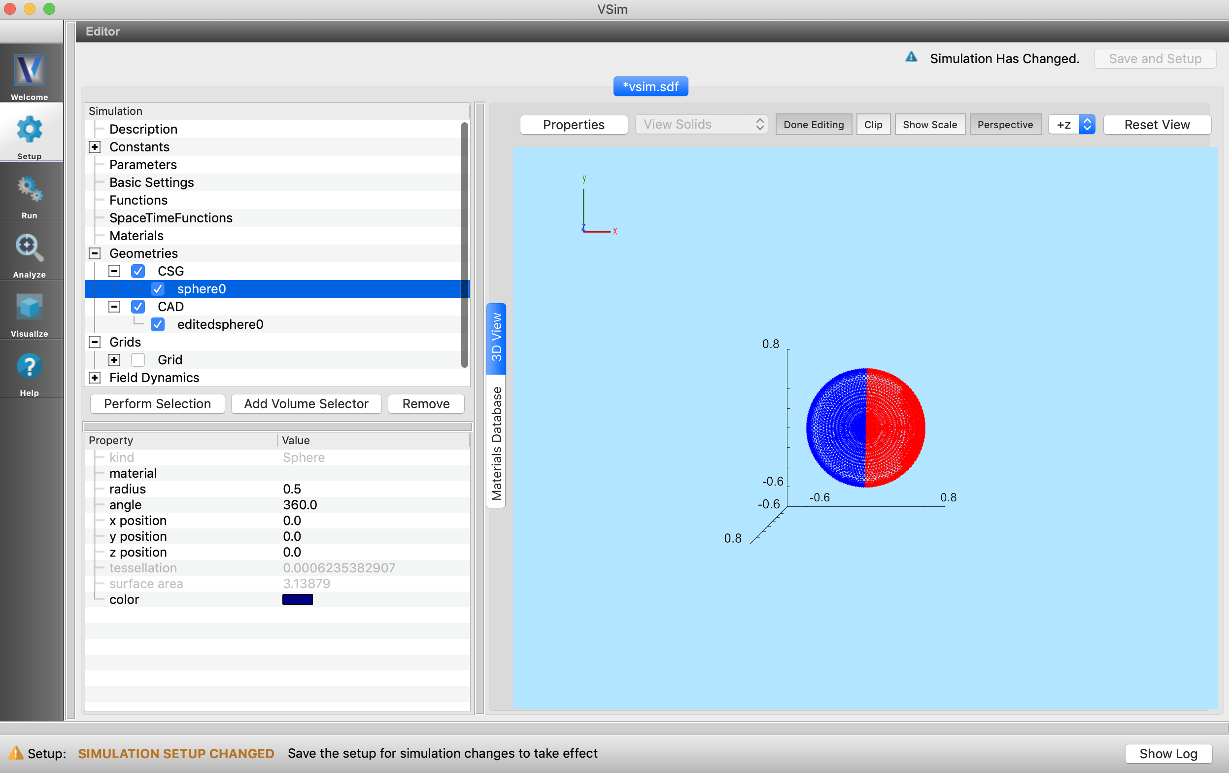
Fig. 66 The Partially Selected Geometry.

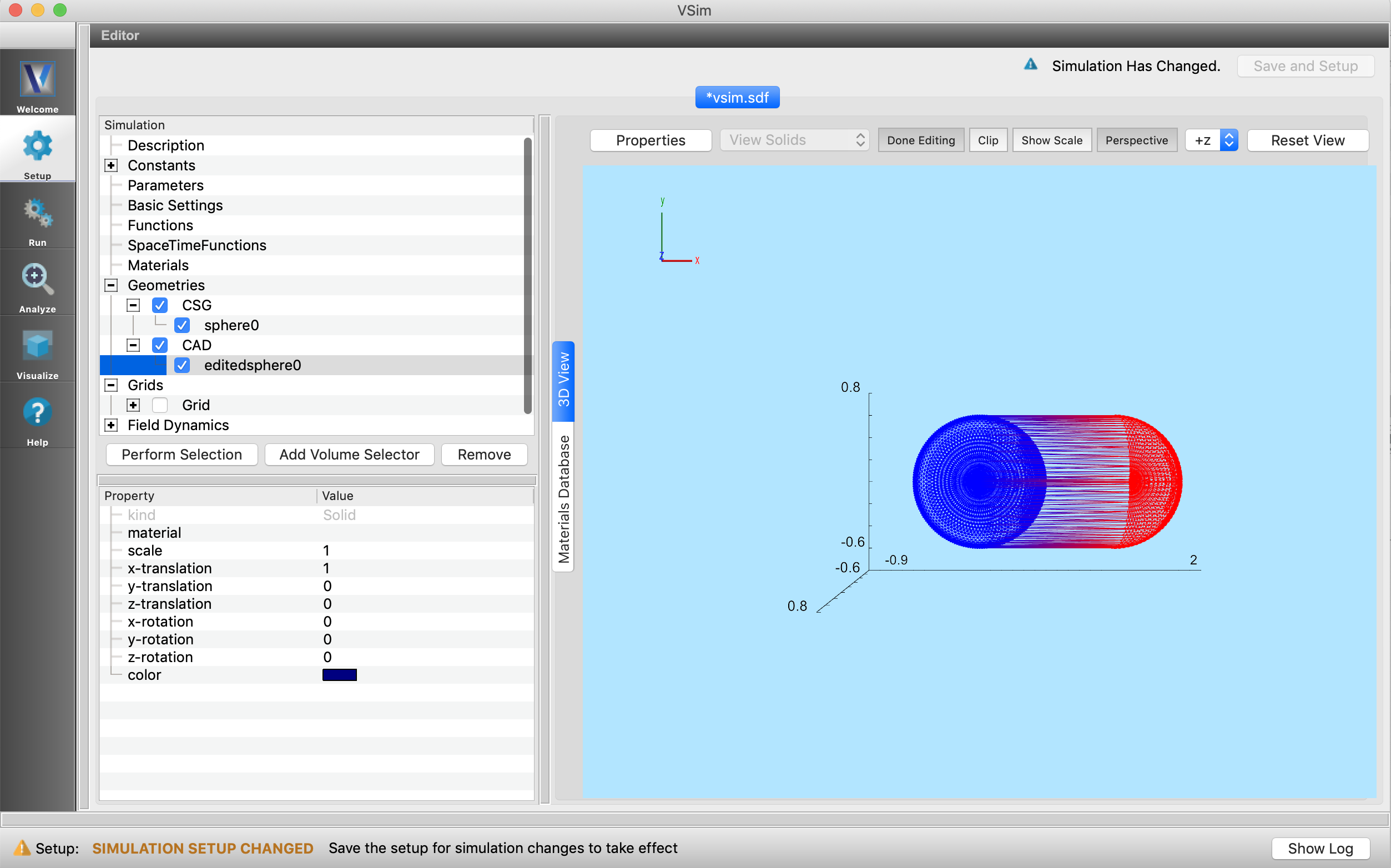
Fig. 67 The Partially Transformed Geometry.

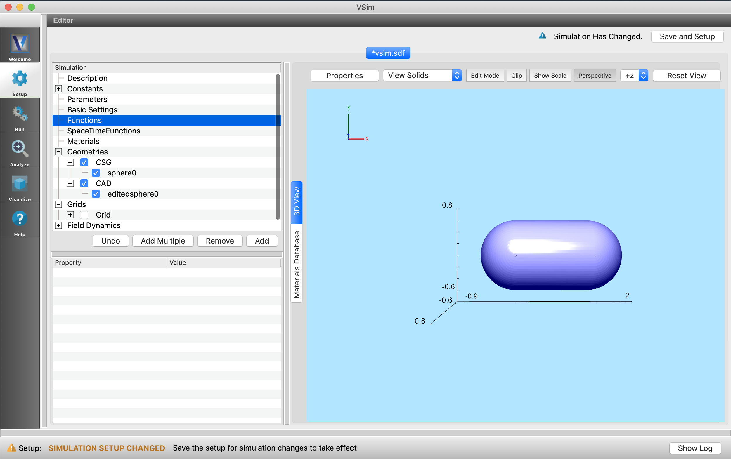
Fig. 68 The Final Geometry.

Navigating

Navigation in 3D space is possible under keyboard and mouse control.

• Rotate

  Holding down the right mouse button and dragging it will rotate the camera position around the object being viewed.

• Pan

  Holding down the left mouse button and the Shift key pans the view in a plane without rotating the viewed object.

• Zoom

  Using the mouse wheel, the view can be zoomed in or out. If the system does not have a mouse wheel, then holding down the left mouse button and the Control key and moving the mouse up and down will also zoom in and out.

Database View

The Database View is for viewing and adding materials to your simulation. Initially, the Database View is blank, but upon importing a materials (.vmat) file, the view is populated with a table of data from the file. See Fig. 69.

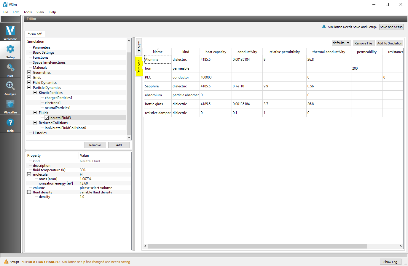
Fig. 69 The Database view

You can switch between files, if more than one file is open, by changing the left drop-down menu. You can remove a file by first switching to the file you would like to close, and then clicking on the Remove File button.

You can add materials to your simulation by highlighting the particular material you are interested in, and then clicking on the Add to Simulation button.

For more information on materials, please see Materials.