Dielectric Wall Wakefield Acceleration (dielectricwallaccelerationt.pre)
Keywords:
- electron driven, plasma wakefield, CLARA, PARS, AWAKE
Problem description
An alternative to a full particle in cell approach for accelerator computations is to use a prescribed beam, that is to set the J field directly without using a vector deposition of the current associated with the charge. This is demonstrated in this example which computes the wakefields in a dielectric lined waveguide. The electron beam initializes the field using a custom python technique, which can be adapted for cases where the Poisson solve might not be appropriate (due to memory limitations for example) then the fields (and effective) particles are evolved using FDTD. We launch the electron beam from x=0 in the positive x direction. The primary bunch generates a region of high field into which one might inject and accelerate a second bunch of charged particles. This simulation broadly follows the approach reported on in [MPSC11]
Opening the Simulation
The Dielectric Wall Wakefield Acceleration example is accessed from within VSimComposer by the following actions:
Select the New → From Example… menu item in the File menu.
In the resulting Examples window expand the VSim for Plasma Acceleration option.
Expand the Beam Driven Acceleration (text-based setup) option.
Select Dielectric Wall Wakefield Acceleration (text-based setup) and press the Choose button.
In the resulting dialog, create a New Folder if desired, and press the Save button to create a copy of this example.
The basic variables of this problem should now be alterable via the text boxes in the left pane of the Setup Window, as shown in Fig. 467.
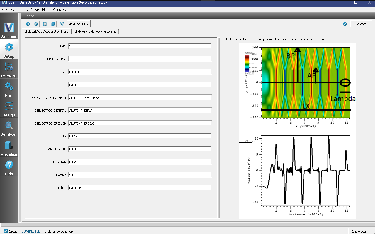
Fig. 467 Setup Window for the Dielectric Wall Wakefield Acceleration example.
Input File Features
The simulation setup consists of an electromagnetic solver using the Yee algorithm and takes advantage of a prescribed current source to avoid computationally intensive particle pushes. The ‘top’ and ‘bottom’ y extents of the simulation are metal, and we see the behavior in a dielectric lined waveguide, using a first order accurate dielectric algorithm for the walls.
BPis the beampipe half-widthAPis the dielectric aperture half-widthDIELECTRIC_EPSILONallows the user to experiment with different materialsLXsets the length of the structure and simulationGammasets the relativistic velocity of the beam to be used.
Inside the .pre file, which you can reach by pressing View Input File, there are various other settings for modelling this with a laser drive, or with PIC particles.
Running the Simulations
After performing the above actions, continue as follows:
Proceed to the Run Window by pressing the Run tab in the left column of buttons.
To run the file, click on the Run button in the upper left corner of the Logs and Output Files pane. You will see the output of the run in the right pane. This is shown in Fig. 468. The run has completed when you see the output, “Engine output has completed successfully.”
Running in 2D, you can expect a 2 core laptop to take a few tens of minutes at the default resolution and run time.
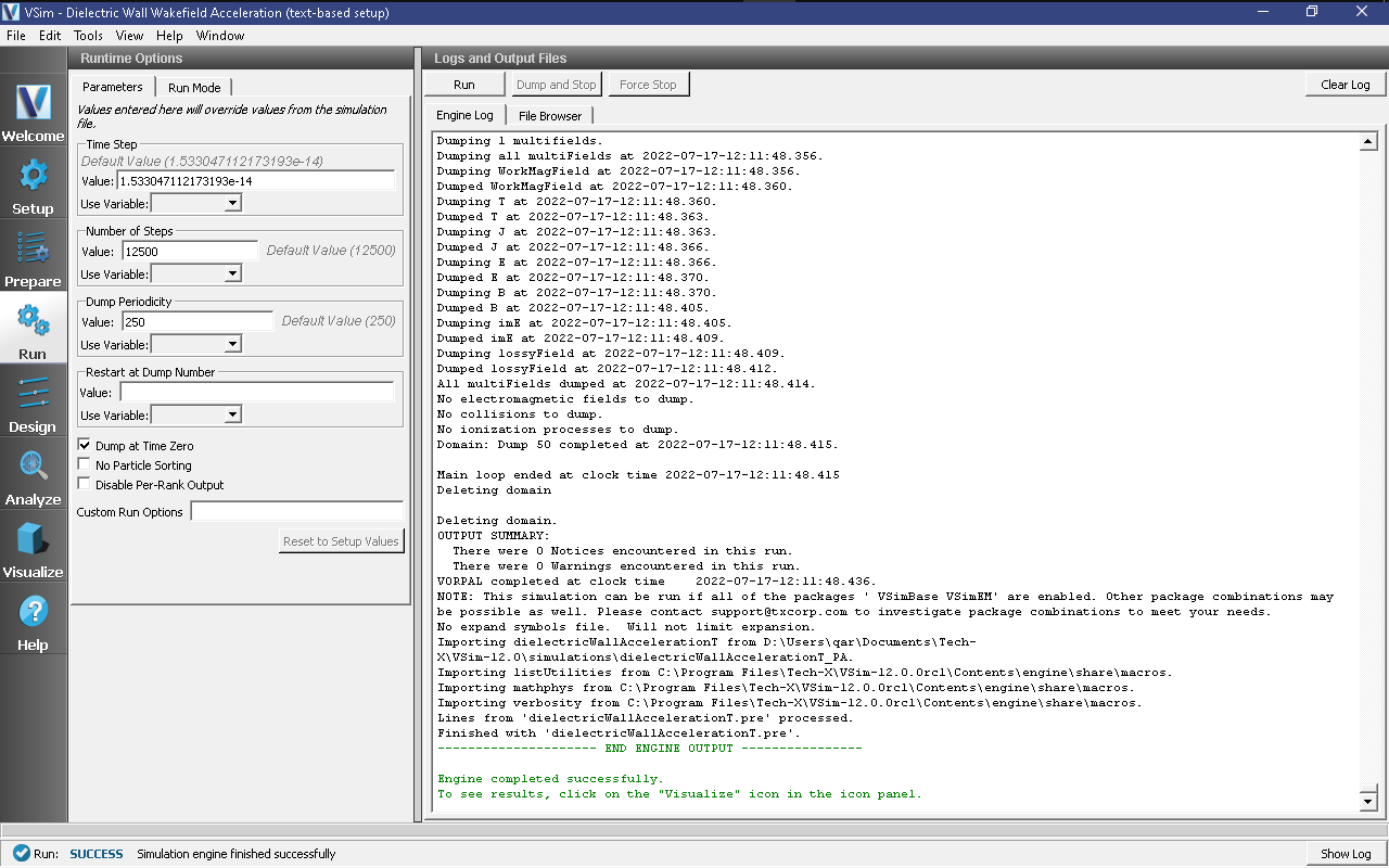
Fig. 468 The Run Window.
Visualizing the Output
After performing the above actions, continue as follows:
Proceed to the Visualize Window by pressing the Visualize tab in the left column of buttons.
View the electric field generated by the plasma as shown in Fig. 469 by doing the following:
Switch to Field Analysis in the Data View Controls pane
Set the Field to E_x
Choose the Horizontal tab in Lineout Settings set the intercept to zero, and click Perform Lineout
Below Perform Lineout in the Layout: drop down menu, Select stacked 2d/1d view.
Check the Auto Reset buttons on both the 2d and the Lineout plots. Sometimes it is necessary to expand the plot size in order for the box to appear. You can do this by pulling the divider between “Visualization Controls” and “Visualization Results” to the left and hiding it. Both the 2d and the Lineout plots should be larger now.
Move the dump slider forward in time.
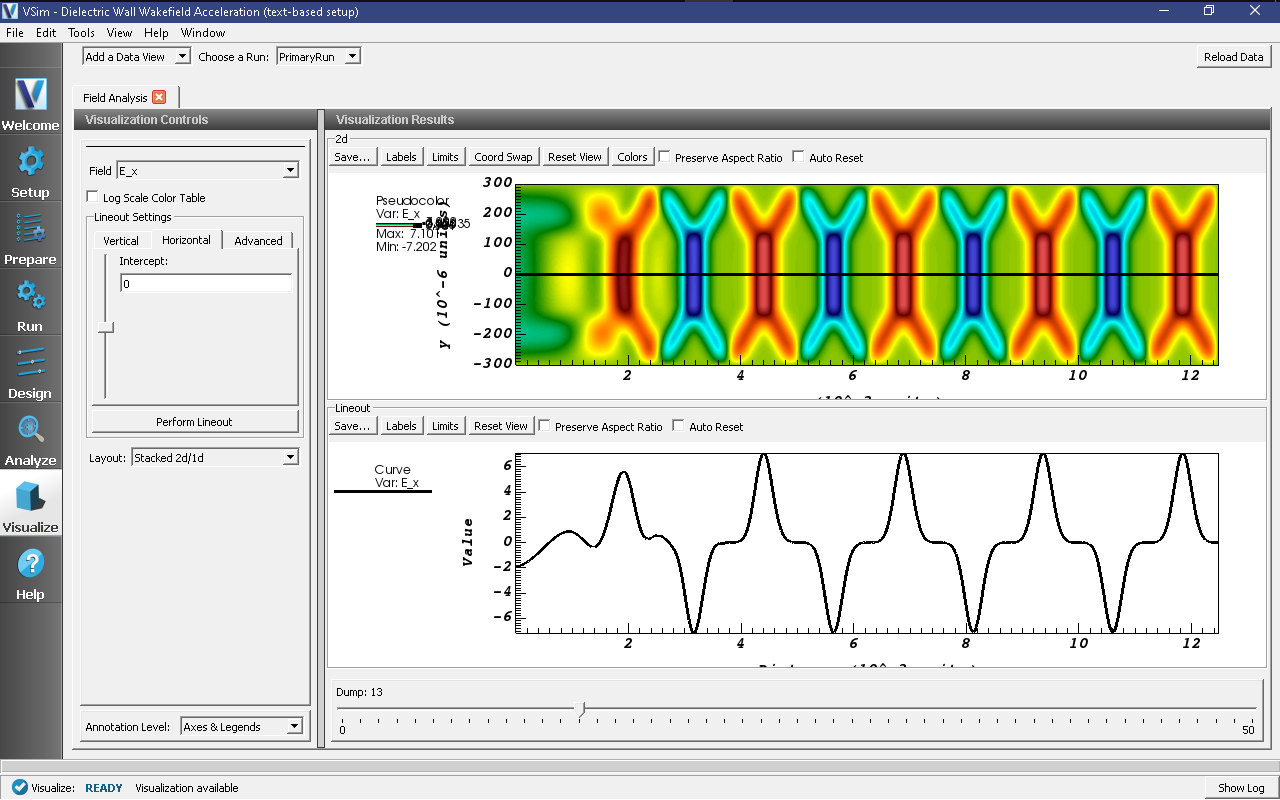
Fig. 469 Visualization of the longitudinal electric field as a color contour plot and longitudinal lineout.
Further experiments
There are two bunch shapes provided to start with, you can look at the effect of harmonics in the bunch in the longitudinal field output. There is also a commented block of code that can be switched in that shifts the dielectric into the domain a little, so one can see the process of the electrons beam forming the pattern.
Also, one may add a species propagating from the left hand side to witness the wake, and observe the behavior of particles in or out of phase with the wake.