extractModes.py
This analyzer extracts the frequencies and modes of a field from time-series data using the Filter Diagonalization Method (FDM) [WC08]. It is useful for simulations in which one has modes of well defined frequencies, and where only a modest number (<~20) of modes are excited. An example simulation would be that of electromagnetic oscillations rung up by a narrow frequency band of excitation current.
- -s <simname>, --simulationName=<simname>
(string, required)
<simname> is the name of the simulation to be analyzed. The file extension should NOT be included in this text field.
- -f <fld>, --field=<fld>
(string, required)
<fld> is the name of the field (E or B) to which we apply the FDM.
- -b <bd>, --beginDump=<bd>
(int, required, default = 2)
<bd> is the initial dump number used by the FDM method. This must be after the source excitation has been turned off.
- -e <ed>, --endDump=<ed>
(int, required, default = 10)
<ed> is the ending dump number used by the FDM method. This is exclusive, so if
beginDump= 10 andendDump= 15, FDM will use dumps 10, 11, 12, 13, and 14.
- -m <nummodes>, --nModes=<nummodes>
(int, required, default = 5)
<nummodes> is the number of modes to find in the frequency range.
- -t <samptype>, --sampleType=<samptype>
(int, optional, default = 0)
<samptype> Sampling type (0 for uniform, 1 for random), which determines how the modes are sampled on the grid.
- -u <unipts>, --numberUniformPts=<unipts>
(int, optional, default = 10)
<unipts> is the number of points to sample uniformly in each direction (required if <samptype> = 0, otherwise ignored).
- -r <ranpts>, --numberRandomPts=<ranpts>
(int, optional, default = 100)
<ranpts> is the number of points to sample randomly (required if <samptype> = 1, otherwise ignored).
- -c, --construct
(int, optional, default = 1, to construct)
Whether to construct modes.
- -w, --overwrite
(flag)
Whether a dataset or group should be overwritten if it already exists.
Output
This analyzer outputs the data in columns. The frequency is in the column labeled freq [Hz] (eigenmode frequency), the inverse quality factor is in the column labeled invQ, and the singular value decomposition index is in the column labeled SVD.
This analyzer also creates new eigenmode fields that may be
viewed in the VSimComposer Visualize tab. For example, a
simulation with an electric field E would have the scalar
fields E_x/y/z (eigenE) in addition to the electric fields
E_x/y/z (E).
If you are running this analyzer from the UI, and the output dataset file already exists, then it will be overwritten each time the analyzer is run, unless you uncheck the Overwrite Existing Files box near the bottom of the Analysis Results pane.
If you are running the analyzer from the command line, the dataset will not be overwritten
unless the -w, or --overwrite flag is specified on the command line.
The results of your analyzer may not be written into the output file if you have not specified the overwrite option to be True.
Usage Recommendations
Current Source
It is recommended that the current source used to excite a cavity take the following form:
as depicted in Fig. 634
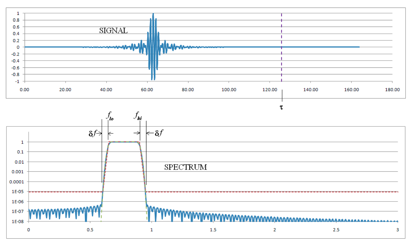
Fig. 634 Time and frequency space plots of current source
\(I_0 = I\left(\tau/2\right)\) is the maximum current, \(\tau = 2 u^2 / \pi \delta f\) is the duration of the excitation, \(f_{lo}\) and \(f_{hi}\) are respectively the lower and upper frequency limits of the excitation, \(H\) is the Heaviside function, and \(\delta f\) and \(u\) together control the steepness of the frequency spectrum near \(f_{lo}\) and \(f_{hi}\). The ratio of the frequency space current source amplitude for frequencies outside the interval \(\left[f_{lo}-\delta f,f_{hi}+\delta f\right]\) to those inside the interval can be specified by the parameter \(u\) with the following table:
Ratio |
\(u\) |
|---|---|
\(10^{-4}\) |
2.76 |
\(10^{-5}\) |
3.13 |
\(10^{-6}\) |
3.46 |
\(10^{-7}\) |
3.77 |
\(10^{-8}\) |
4.06 |
The input option --beginDump should be set to a dump for which \(t > \tau\).
Frequency Option
There are some rough guidelines for choosing a suitable value of the parameter \(\delta f\):
If examining the low end of a spectrum, where the mode density is not too high, \(\delta f \approx f_{lo} / 4\) is reasonable.
If examining a narrow range of frequencies at the high end of a spectrum, \(\delta f \approx \left(f_{hi}-f_{lo}\right)/4\) is reasonable.
If intentionally trying to exclude modes outside of, but close to, the nominal spectrum from \(f_{lo}\) to \(f_{hi}\), a smaller value of \(\delta f\) may be necessary. If \(\delta f\) is too small, however, heavily damped modes may disappear entirely.
If anticipating modes with loss parameter \(Q_m\) near frequency \(f_m\), \(\delta f\) should satisfy \(\delta f \ge 2 f_m / Q_m\) to ensure the modes are present after the excitation turns off.
For loss-less systems where \(Q \rightarrow \infty\), \(\delta f\) may be as small as desired.
Missing modes may occur if the duration of the simulation is too large, causing modes with finite decay to disappear (in which case, \(\delta f\) should be increased).
Dump Interval and Number of Dumps
The following are some guidelines for choosing the dump interval
and number of dumps, --endDump - --beginDump.
The dump interval should be smaller than half a period of the highest frequency present.
The number of dumps should cover at least one cycle of the smallest frequency present.
There should be at least three times as many dumps as the number of modes found.