Y Splitter (ySplitter.sdf)
Keywords:
- S Parameter, Mode Launcher, MAL, Guided Mode, Photonic Device, Semiconductor
Problem Description
The Y Splitter makes use of a gds file of a passive photonic device, intended to split the power of a single incoming wave into two separate branches.
The device itself is silicon, surrounded by silicon dioxide.
This examples makes use of a “Photonics simulation template” intended to allow for rapid setup of any passive photonic device, provided the ports are aligned with the X-Axis. Matched Absorbing Layers (MALs) are used to dampen the E, B and D fields near the boundary of the simulation.
The fundamental guided mode profile is launched as a wide band pulse in the input waveguide. This mode is imported from the file port1LowRes_EigenD_0.vsh5, produced by the computeWaveguideModes.py analyzer. We will use the computeSParamsViaOverlapIntegral.py analyzer to determine the transmission coefficients at the two exit ports of the device.
This simulation out of the box is set to a minimal resolution, allowing for a faster simulation time, with 8 cells per wavelength (in Silicon) used. For typical use cases a value of 12-18 cells per wavelength is recommended.
This simulation can be performed with a VSimEM license.
Opening the Simulation
The Y Splitter example is accessed from within VSimComposer by the following actions:
Select the New → From Example… menu item in the File menu.
In the resulting Examples window expand the VSim for Electromagnetics option.
Expand the Photonics option.
Select Y Splitter and press the Choose button.
In the resulting dialog, create a New Folder if desired, and press the Save button to create a copy of this example.
All of the properties and values that create the simulation are available in the Setup Window as shown in Fig. 304. You can expand the tree elements and navigate through the various properties. The right pane shows a 3D view of the geometry, as well as the grid, if actively shown. To show or hide the grid, expand the Grid element and select or deselect the box next to Grid.
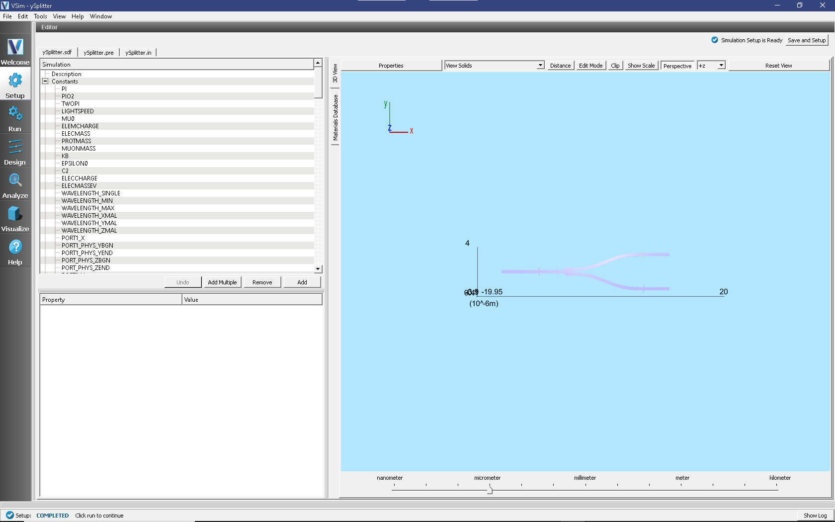
Fig. 304 The Setup window for the y splitter example showing the imported gds file.
Simulation Properties
This example contains a number of Constants defined to make the simulation easily modifiable. These are also intended to be reset for a different gds file and will redefine the simulation size and parameters
General Simulation Constants:
WAVELENGTH_SINGLE = Used for a single wavelength simulation and calculation of simulation information based on wavelength.
WAVELENGTH_MIN = Minimum wavelength for a multi-wavelength simulation.
WAVELENGTH_MAX = Maximum wavelength for a multi-wavelength simulation.
WAVELENGTH_XMAL = Number of wavelengths of MAL in the X-direction.
WAVELENGTH_YMAL = Number of wavelengths of MAL in the Y-direction.
WAVELENGTH_ZMAL = Number of wavelengths of MAL in the Z-direction.
PORT1_X = Location of port 1 (excitation port) on the X-axis.
PORT1_PHYS_YBGN = Beginning of Port 1 on the Y-axis.
PORT1_PHYS_YEND = End of Port 1 on the Y-axis.
PORT_PHYS_ZBGN = Beginning of all ports on the Z-axis
PORT_PHYS_ZEND = End of all ports on the Z-axis
PORT2_X = Location of port 2 on the X-axis.
PORT2_PHYS_YBGN = Beginning of Port 2 on the Y-axis.
PORT2_PHYS_YEND = End of Port 2 on the Y-axis.
PORT3_X = Location of port 3 on the X-axis.
PORT3_PHYS_YBGN = Beginning of Port 3 on the Y-axis.
PORT3_PHYS_YEND = End of Port 3 on the Y-axis.
PORT4_X = Location of port 4 on the X-axis.
PORT4_PHYS_YBGN = Beginning of Port 4 on the Y-axis.
PORT4_PHYS_YEND = End of Port 4 on the Y-axis.
PORT5_X = Location of port 5 on the X-axis.
PORT5_PHYS_YBGN = Beginning of Port 5 on the Y-axis.
PORT5_PHYS_YEND = End of Port 5 on the Y-axis.
PORT1_LEFT_SIDE = Set to 1 if on the left side of the simulation, -1 if on the right.
PORT2_LEFT_SIDE = Set to 1 if on the left side of the simulation, -1 if on the right.
PORT3_LEFT_SIDE = Set to 1 if on the left side of the simulation, -1 if on the right.
PORT4_LEFT_SIDE = Set to 1 if on the left side of the simulation, -1 if on the right.
PORT5_LEFT_SIDE = Set to 1 if on the left side of the simulation, -1 if on the right.
MIN_Y_COORDINATE = Minimum Y coordinate of the component, used if less than any of the ports.
MAX_Y_COORDINATE = Maximum Y coordinate of the component, used if greater than any of the ports.
CELLS_PER_WAVELENGTH_AXIAL = Number of cells per wavelength (in Silicon) along the X axis.
CELLS_PER_WAVELENGTH_CROSSSECTION = Number of cells per wavelength (in Silicon) along the Y and Z axis.
This simulation applies a wide frequency band signal to the fundamental spatial mode profile. The signal is defined under SpaceTimeFunctions and then assigned under Field Dynamics, Fields, port1
The Materials section contains just Silicon and Silica. This section is where one can add or edit materials that get attached to CSG objects. These Materials contain the relative permittivity.
In Field Dynamics there are FieldBoundaryConditions which set the boundary conditions of the simulation. In photonics simulations, Matched Absorbing Layers (MALs), are the most stable boundary conditions for preventing reflections.
Under Basic Settings you can see that the dielectric solver is set to permittivity averaging. This feature enables second order accuracy for simulations using dielectrics.
GDSII File Import
The GDS File has already been imported, however this example serves as a good demonstration of how to do so
It may be imported like any other CAD file, however a second dialog box will appear, shown below.
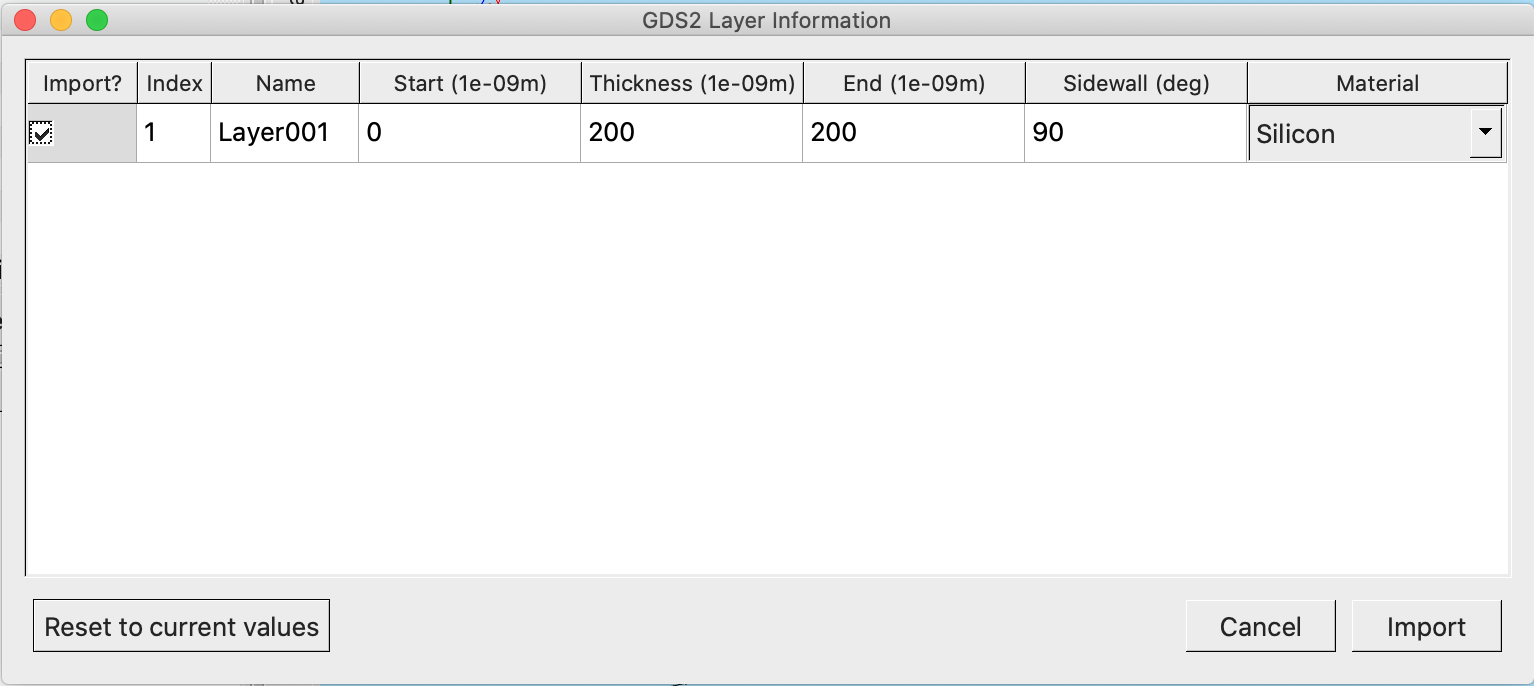
Fig. 305 GDS layer selection.
This allows for selection if the layer should be imported, it’s starting position on the Z axis, and thickness. Sidewall angles can also be set however this is a feature that is still under active development at this time and is recommended to be kept at 90 degrees.
Running the Simulation
When you have saved the setup, continue as follows:
Proceed to the Run Window by pressing the Run button in the left column of buttons.
When you are finished setting run parameters, click on the Run button in the upper left corner of the right pane.
You will see the output of the run in the right pane. The run has completed when you see the output, “Engine completed successfully.” As seen in Fig. 306.
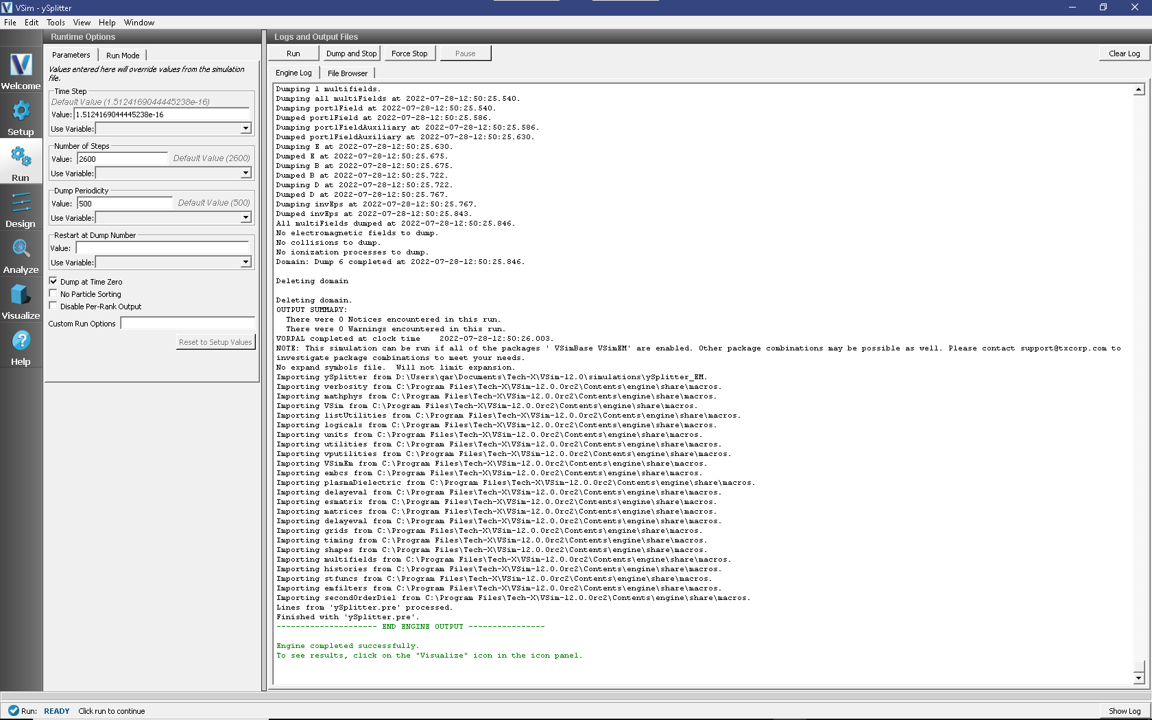
Fig. 306 Run window at completion.
Analyzing the Results
Using post analysis scripts, one can extract the transmission coefficients. This simulation uses 4 “EM Field on Plane” histories (Port1, Port2, Port3, Port1Enter) and this data is used to calculate S parameters between these 4 locations using the analysis script computeSParamsViaOverlapIntegral.py.
Port1Enter is described in Further Experiments.
Follow these steps:
Proceed to the Analyze Window by clicking the Analyze button on the left.
Select computeSParamsViaOverlapIntegral.py and click Open under the list.
Now update the analyzer fields accordingly.
maxWavelength: 1.7e-6 (or use the corresponding parameter from the setup)
minWavelength: 1.4e-6 (or use the corresponding parameter from the setup)
inPlane: Port1_History (or Port1Enter_History)
outPlane: Port2_History (or Port3_History)
The remaining parameter default values will work. Hit the Analyze button in the top tight corner. After a successful run the window should resemble Fig. 307.
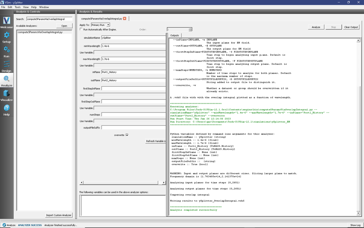
Fig. 307 Analyze window with output from computeSParamsViaOverlapIntegral.py.
Visualizing the results
After performing the above actions proceed to the Visualize Window by pressing the Visualize button in the left column of buttons.
Near the top left corner of the window, select 1-D Fields from the Add a Data View drop-down.
In the Plot Control panel select the Port2 and Port3 SParams data for graph 1.
Set the other Graphs to None
The results are shown in Fig. 308. As expected, we see equivalent power split between the two ports across the wavelength range
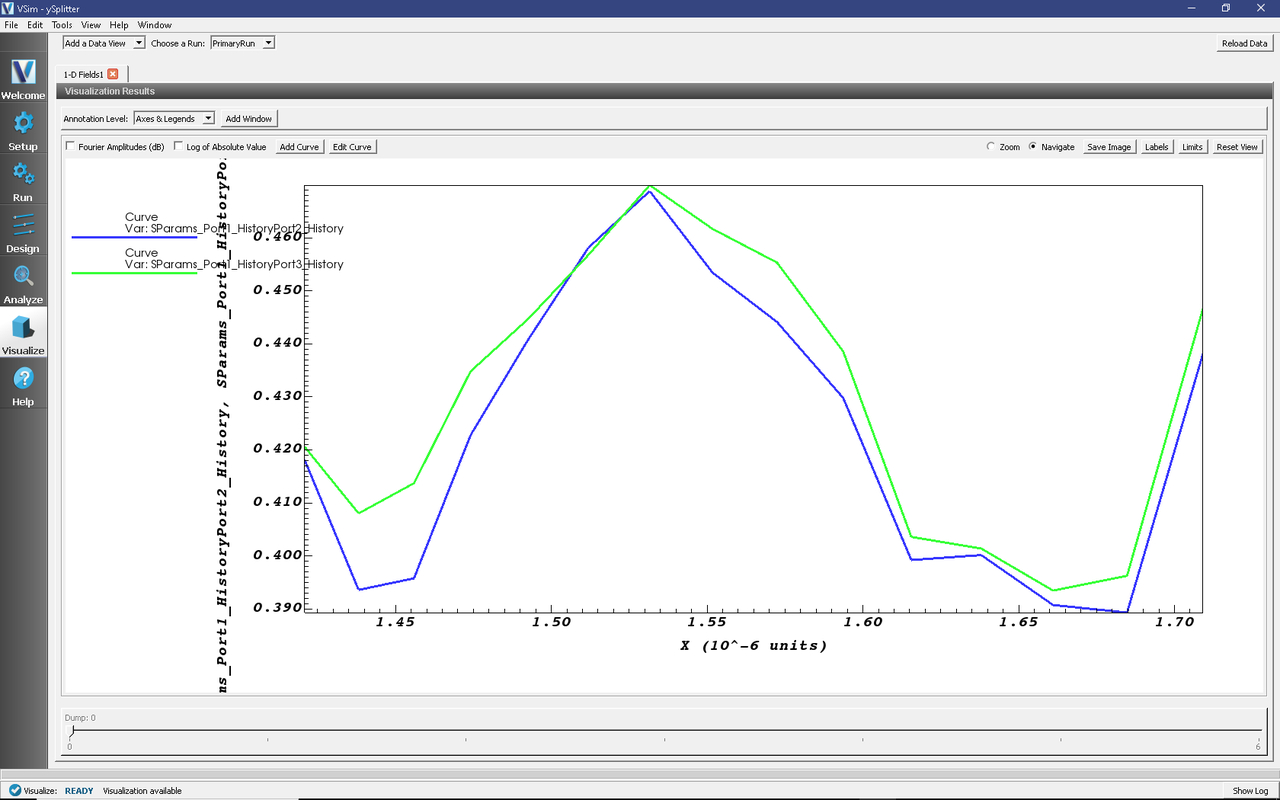
Fig. 308 Visualization of the s-parameters.
Further Experiments
This example comes with a second port “Port1Enter” Calculating the modes from this port to ports 2/3 will show a slightly higher transmission coefficient. This is because the mode solve is somewhat inaccurate at a low resolution so some loss occurs in the first few wavelengths. Try increasing the resolution, recalculating the mode and these two values should grow closer in agreement.
This example can be easily adapted for different GDS files.