Microring Resonator with Gaussian Launcher (ringResonatorGaussianMode.sdf)
Keywords:
- Ring Resonator, Mode Launcher, MAL, Guided Mode, Photonic Device, Semiconductor
Problem Description
The Ring Resonator consist of two straight Silicon waveguides and a Silicon waveguide ring that sits between the straight waveguides. All three waveguides rest on top of a Silicon Dioxide slab. The rest of the simulation domain is set to vacuum. Matched Absorbing Layers (MALs) are used to dampen the E, B and D fields near the boundary of the simulation.
The approximate fundamental guided mode profile is launched as a wide band pulse in the input waveguide. This mode is a simple 2D Gaussian distribution centered at the center of the waveguide. This approximate mode is accurate enough for this simulation. The exact mode can be calculated using the computeWaveguideModes analyzer. To go through the mode solve process check out the Multimode Fiber Mode Calculation example. We will use the computeSParamsViaOverlapIntegral.py analyzer to determine the transmission coefficients at the thru-port and drop port.
This simulation can be performed with a VSimEM license.
Opening the Simulation
The Ring Resonator example is accessed from within VSimComposer by the following actions:
Select the New → From Example… menu item in the File menu.
In the resulting Examples window expand the VSim for Electromagnetics option.
Expand the Photonics option.
Select Ring Resonator and press the Choose button.
In the resulting dialog, create a New Folder if desired, and press the Save button to create a copy of this example.
All of the properties and values that create the simulation are available in the Setup Window as shown in Fig. 299. You can expand the tree elements and navigate through the various properties. The right pane shows a 3D view of the geometry, as well as the grid, if actively shown. To show or hide the grid, expand the Grid element and select or deselect the box next to Grid.
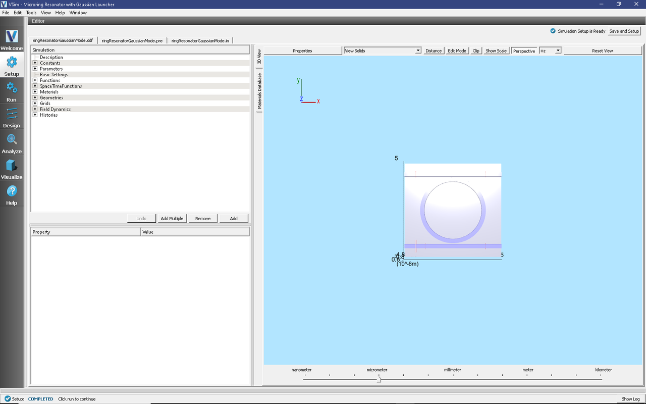
Fig. 299 The Setup window for the ring resonator example showing the external mode launching field.
Simulation Properties
This example contains a number of Constants defined to make the simulation easily modifiable.
General Simulation Constants:
RESOLUTION_XY = the inverse of the number of cells per wavelength
RESOLUTION_Z = the inverse of the number of cells per waveguide height in the z dimension
WAVELENGTH_CENTER = the central wavelength used in the excitation
WIDTH_EXCITATION = the width in wavelength space of the wide band signal
RADIUS_RING = radius of the ring
WIDTH_WAVEGUIDE = Width of waveguides
HEIGHT_WAVEGUIDE = Height of waveguides
WIDTH_GAP = Width of the gap between ring and waveguides
This simulation applies a wide frequency band signal to the approximate fundamental spatial mode profile. The signal is defined under SpaceTimeFunctions and then assigned under Field Dynamics, CurrentDistributions, generalDistributedCurrent as shown in Fig. 299.
The Materials section contains just Silicon and Silica. This section is where one can add or edit materials that get attached to CSG objects. These Materials contain the relative permittivity.
In Field Dynamics there are FieldBoundaryConditions which set the boundary conditions of the simulation. In photonics simulations, Matched Absorbing Layers (MALs), are the most stable boundary conditions for preventing reflections.
Under Basic Settings you can see that the dielectric solver is set to permittivity averaging. This feature enables second order accuracy for simulations using dielectrics.
Running the Simulation
When you have saved the setup, continue as follows:
Proceed to the Run Window by pressing the Run button in the left column of buttons.
When you are finished setting run parameters, click on the Run button in the upper left corner of the right pane.
You will see the output of the run in the right pane. The run has completed when you see the output, “Engine completed successfully.” As seen in Fig. 300.
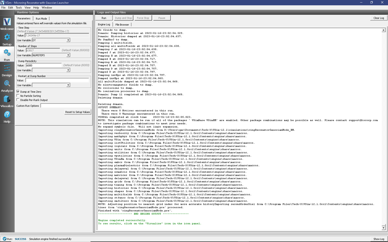
Fig. 300 Run window at completion.
Analyzing the Results
Using post analysis scripts, one can extract the transmission coefficients. This simulation uses 4 “EM Field on Plane” histories (slab0-slab4) and this data is used to calculate S parameters between these 4 locations using the analysis script computeSParamsViaOverlapIntegral.py.
Follow these steps:
Proceed to the Analyze Window by clicking the Analyze button on the left.
Select computeSParamsViaOverlapIntegral.py and click Open under the list.
Now update the analyzer fields accordingly.
maxWavelength: 1.7e-6 (or use the corresponding parameter from the setup)
minWavelength: 1.4e-6 (or use the corresponding parameter from the setup)
inPlane: slab0
outPlane: slab1 (or slab3)
outSLabB: slab1 (or slab3)
outputFileSuffix: S01 (or S03)
The remaining parameter default values will work. Hit the Analyze button in the top right corner. After a successful run the window should resemble Fig. 301. Continue by analyzing the drop-port. To do this change the outSlabE and outSlabB fields to slab3_E and slab3_B, respectively.
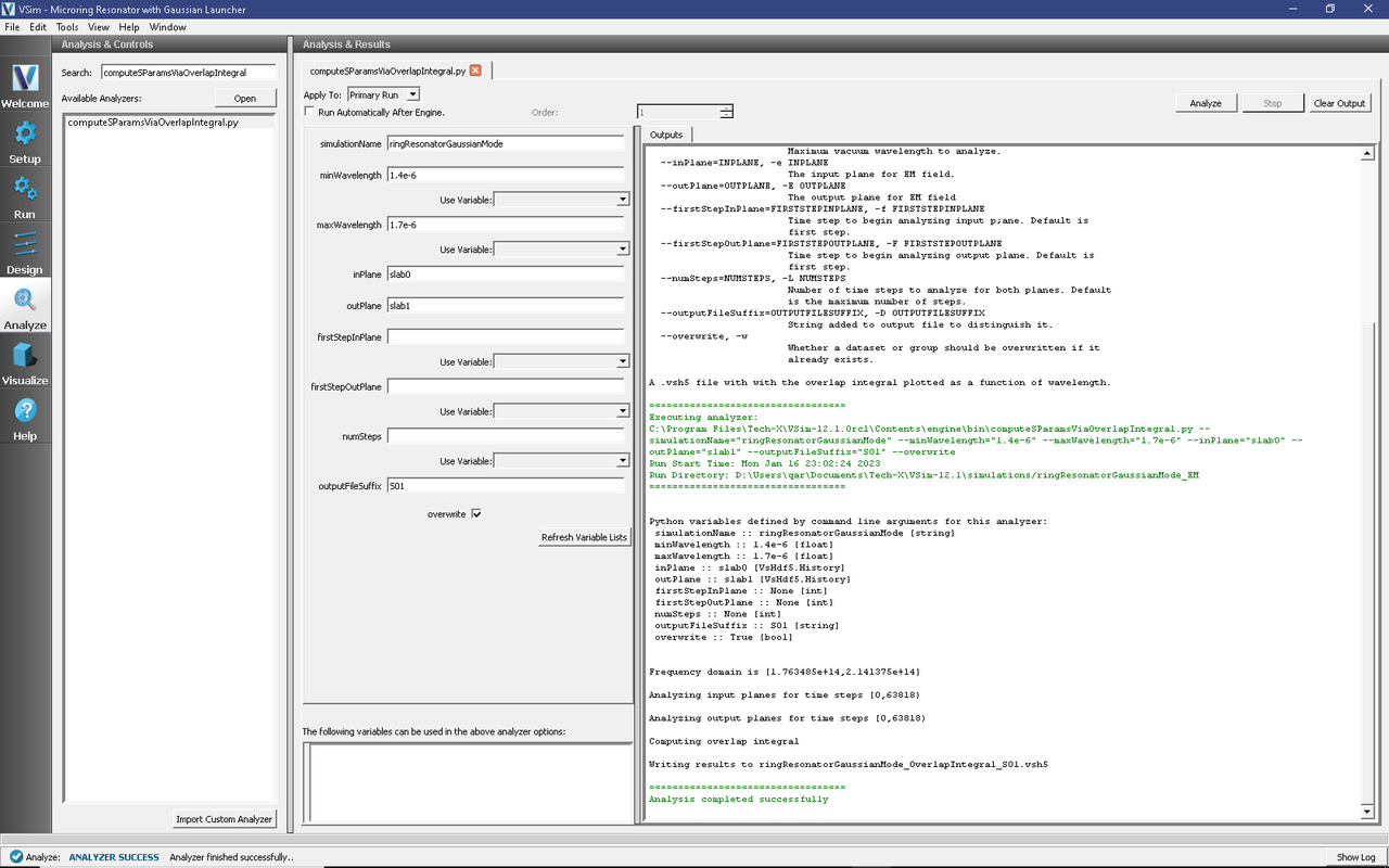
Fig. 301 Analyze window with output from computeSParamsViaOverlapIntegral.py.
Visualizing the results
After performing the above actions proceed to the Visualize Window by pressing the Visualize button in the left column of buttons.
One can visualize the magnetic field by performing the following:
Near the top left corner of the window, select Data Overview from the Add a Data View drop-down.
Expand Scalar Data, then B, then select B_magnitude
In the bottom left, select Clip Plot, and set z=0 in Plane Controls
Finally, move the dump slider on the bottom of the window to watch the light propagate
The results are shown in Fig. 302.
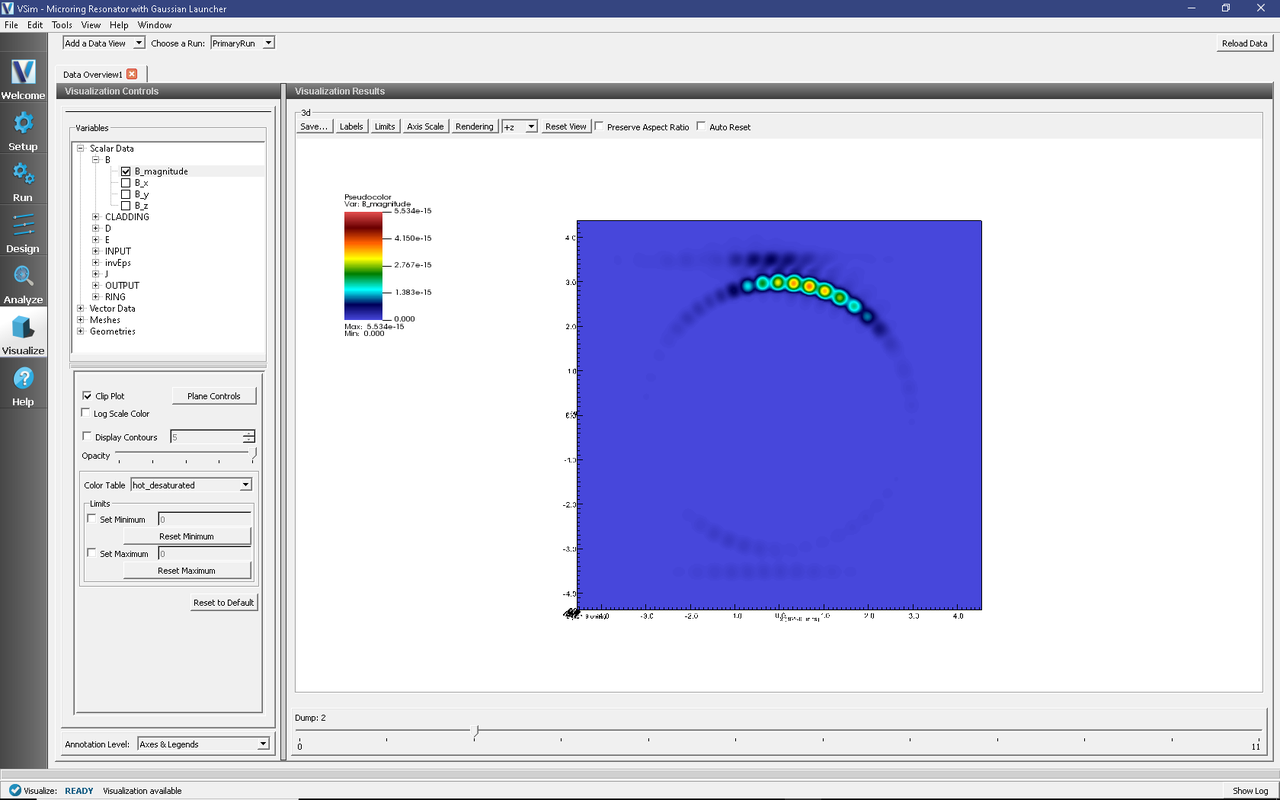
Fig. 302 Visualization of magnetic field.
One can visualize the transmission coefficients by performing the following:
Near the top left corner of the window, select 1-D Fields from the Add a Data View drop-down.
In the Plot Control panel select the Slab1 and Slab3 SParams data for Graphs 1 and 2, respectively.
Set the other Graphs to None
The results are shown in Fig. 303. As expected, we see coupling of resonant wavelengths with the ring.
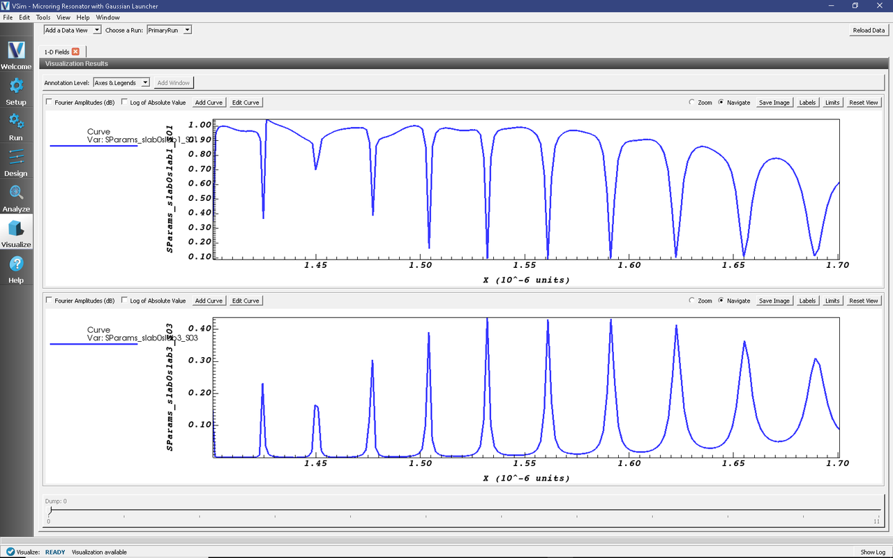
Fig. 303 Visualization of the s-parameters.