Metal Insulator Metal Waveguide using Drude and Lorentz Materials (drudeLorentzMIM.sdf)

Problem Description

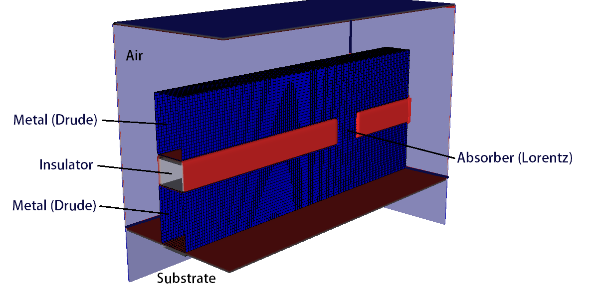
A metal-insulator-metal (MIM) waveguide can propagate optical frequency electromagnetic radiation due to the effective negative index material property of the metal at those frequencies. This negative index material is represented with a time-domain Drude model dielectric, which can support a wide range of frequencies and wide bandwidth.

In addition to the MIM waveguide, a section of the insulator is removed, and replaced with a resonant absorber material, using a time-domain version of the traditional Lorentz material.

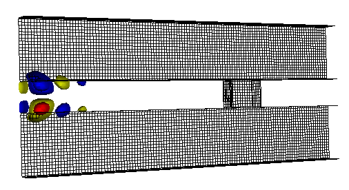
Fig. 289 Longitudinal electric field in the MIM waveguide.

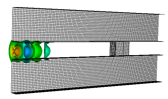
Fig. 290 Transverse electric field in the MIM waveguide.

A spatial gaussian waveform is incident on the edge of the MIM waveguide, coupling to it, and propagating down the length of the waveguide until it encounters the Lorentz material inclusion, where the wave is absorbed. For the incident wave to couple effectively to the MIM waveguide, the spatial size of the gaussian waveform must be a good match to the size of the waveguide, or a large portion of the incident wave will scatter off the structure, rather than coupling to it.

Also, the width, strength, and natural oscillation frequency of the Lorentz material inclusion determines whether the wave is reflected, absorbed, or transmitted when it encounters the inclusion. In this example there is only one Lorentz curve, but multiple Lorentz curves can be added to the simulation.

The length of the MIM waveguide, and the direction of wave propagation is in the x-direction. The width of the waveguide is in the z-direction, and the height of the waveguide is in the y-direction. The waveguide sits atop an insulator substrate, and is surrounded by air. The boundaries of the simulation are ports, allowing for incoming and outgoing waves.

This simulation can be performed with a VSimEM license.

Opening the Simulation

The MIM waveguide example is accessed from within VSimComposer by the following actions:

• Select the New → From Example… menu item in the File menu.

• In the resulting Examples window expand the VSim for Electromagnetics option.

• Expand the Scattering option.

• Select “MIM Waveguide” and press the Choose button.

• In the resulting dialog, create a New Folder if desired, and press the Save button to create a copy of this example.

The Setup Window is now shown with all the implemented physics and geometries, if applicable. See Fig. 291.

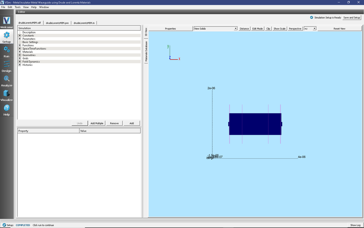
Fig. 291 Setup Window for the drudeLorentzMIM example.

Simulation Properties

The geometry of the waveguide is fully parameterized, allowing for easy adjustment to the waveguide.

A port launcher boundary is used at the lower X boundary to launch a Y polarized wave.

The Drude-Lorentz model dielectric allows for full specification of the Drude model collision and conductivity function, as well as a background conductivity. In this example a single Lorentz model is used with the oscillator, frequency and line width. More Lorentz’s can be added by adding to the vector of these three properties.

The input file also contains a parameter to adjust the spatial resolution of the mesh.

Default parameters are selected to correspond to violet light, a Drude material corresponding to silver, SiO2 insulator (and substrate), and a Lorentz material corresponding to AlAs. The default variable values can be compared to the well known material properties of these materials to establish the exact correspondence to the well-known mathematical descriptions of the Drude and Lorentz models.

Running the simulation

After performing the above actions, continue as follows:

• Proceed to the Run Window by pressing the Run button in the left column of buttons.

• To run the file, click on the Run button in the upper left corner of the window. You will see the output of the run in the right pane. The run has completed when you see the output, “Engine completed successfully.” This is shown in Fig. 292.

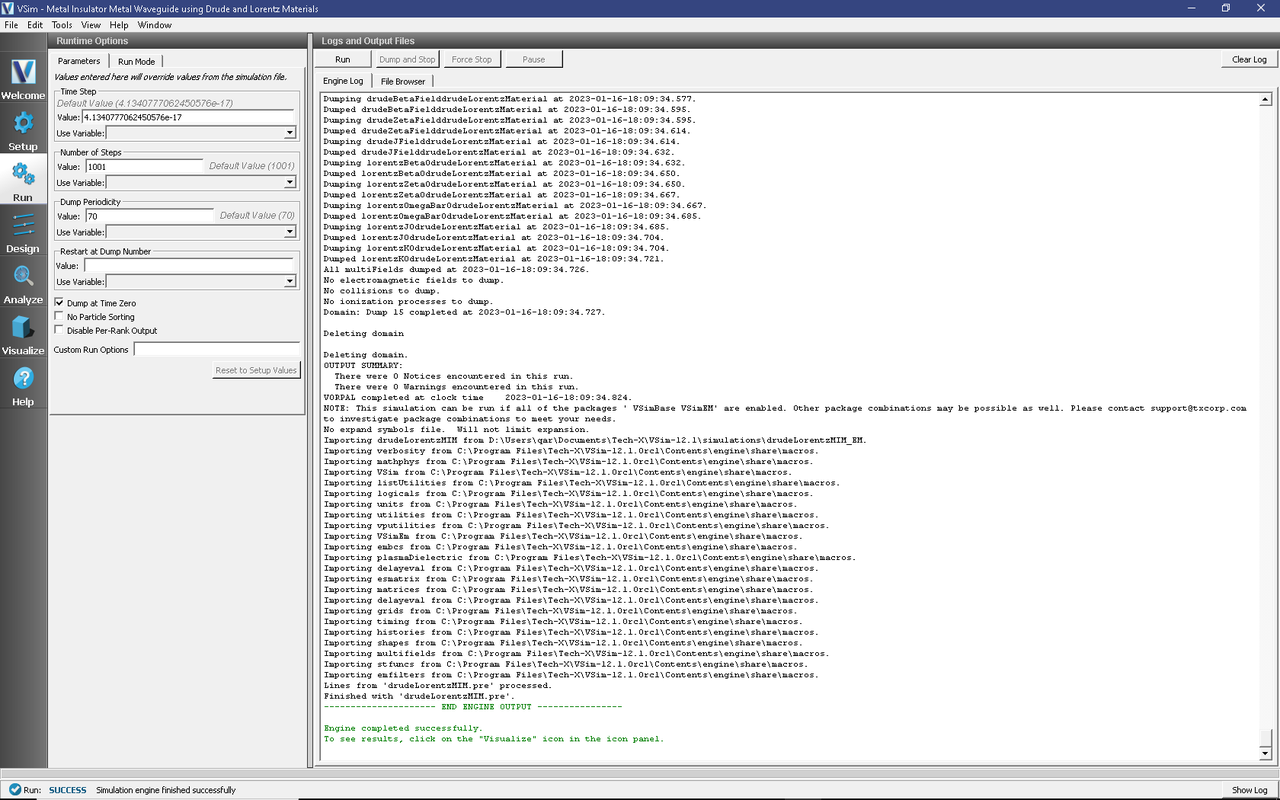
Fig. 292 The Run Window at the end of execution.

Visualizing the results

After performing the above actions, continue as follows:

• Proceed to the Visualize Window by pressing the Visualize button in the left column of buttons.

The results are best viewed by looking at the \(y\) component of the electric field. To view the fields, select Scalar Data variable and check the E_y box. Check the Clip Plot checkbox. Set the minimum value to -0.75 and the maximum value to 0.75. The field is shown in Fig. 293.

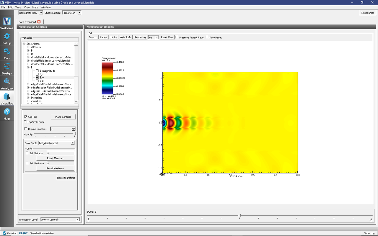
Fig. 293 Visualization of the \(E_y\) field component.

We can see that fields are well coupled between the two metal layers of the waveguide, with only some small leakage, and transient behavior at the entrance. The fields then diminish abruptly at the inclusion, where the wave is mostly absorbed.