Dielectric Waveguide Mode Calculation (dielectricWaveguideModeCalc.sdf)
Keywords:
- Mode Extraction, Photonic Waveguide, Guided Mode, Semiconductor
Problem Description
This example demonstrates the process for extracting the effective index and fields of a guided mode by directly solving an eigenvalue equation. The use of permittivity averaging enables second order accuracy in our solution. The waveguide axis runs parallel to the x-axis, and is surrounded by a background cladding with a greater permittivity. We will run the simulation for 1 step and then use the dielectricWaveguideModeCalc_invEps_0.h5 file to solve for the guided modes using the computeDielectricModes.py analyzer. This analyzer will find the entire basis set of modes for this waveguide and output each into a separate .vsh5 file. These mode files can be used to launch the exact modes into your simulation. This process is shown in the multiModeFiberModeLaunchT example.
Eigenmodes in such a simulation have the form:
The effective index of refraction of a waveguide mode is given by \(\bar{n} = k / k_0\) where \(k_0 = \omega / c\). If the waveguide has index of refraction \(n_w\) and the cladding \(n_c < n_w\), then a guided mode will have a modal index in the range, \(n_c < \bar{n} < n_w\).
This simulation can be performed with a VSimEM license.
Opening the Simulation
To open this example open an instance of VSimComposer and follow the steps below:
Select the New → From Example… menu item in the File menu.
In the resulting Examples window expand the VSim for Electromagnetics option.
Expand the Photonics option.
Select Dielectric Waveguide Mode Calculation and press the Choose button.
In the resulting dialog, create a New Folder if desired, and press the Save button to create a copy of this example.
Simulation Variables
This example contains a number of variables defined to make the simulation easily modifiable.
PERMITTVITY_WAVEGUIDE and PERMITTVITY_BACKGROUND: Relative permittivities of silicon and silica. These constants are used in multiple parameters and in the accompanying Python file for solving the waveguide modes.
WAVELENGTH_VAC: Wavelength of the input signal. This wavelength is also used for the calculation of the fundamental guided mode of the device.
NWAVELENGTH_MAL: Approximate number of wavelengths that can fit in a Matched Absorbing Layer (MAL) region. The thickness of the MAL regions in this example are measured in wavelengths.
The Materials section contains just silicon and silica. The Geometries includes the CSG waveguide and its defining parameters. In Field Dynamics, there are FieldBoundaryConditions and CurrentDistributions to be aware of. In photonics simulations, Matched Absorbing Layers (MALs) are the most stable boundary conditions for preventing reflections. The gaussian approximation is defined under SpaceTimeFunctions and is set to drive the y-component of the currentSource.
Setting up the Simulation
As delivered, the system is set up to generate the data needed to run the computeDielectricModes.py analyzer. To ensure that your simulation has second order accuracy, expand the Basic Settings branch and verify that the dielectric solver field is set to permittivity averaging. This algorithm is a powerful VSim feature. This setting is shown in Fig. 270.
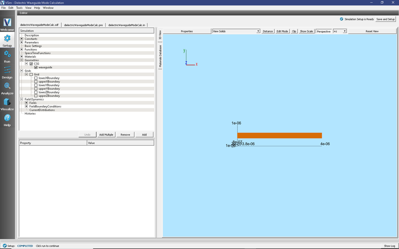
Fig. 270 Choosing the second order accurate, permittivity averaging for the dielectric solver field under Basic Settings.
Running the Simulation
After performing the above actions, continue as follows:
Proceed to the Run Window by pressing the Run button in the left column of buttons. You will be asked to Save. Click Save upon the request to save.
In the left pane change the Number of Steps and Dump Periodicity to 1.
Under Additional Run Options select Dump at Time Zero.
To run the file, click on the Run button in the upper left corner of the right pane. You will see the output of the run in the right pane. The run has completed when you see the output, “Engine completed successfully.” This result is shown in Fig. 271.
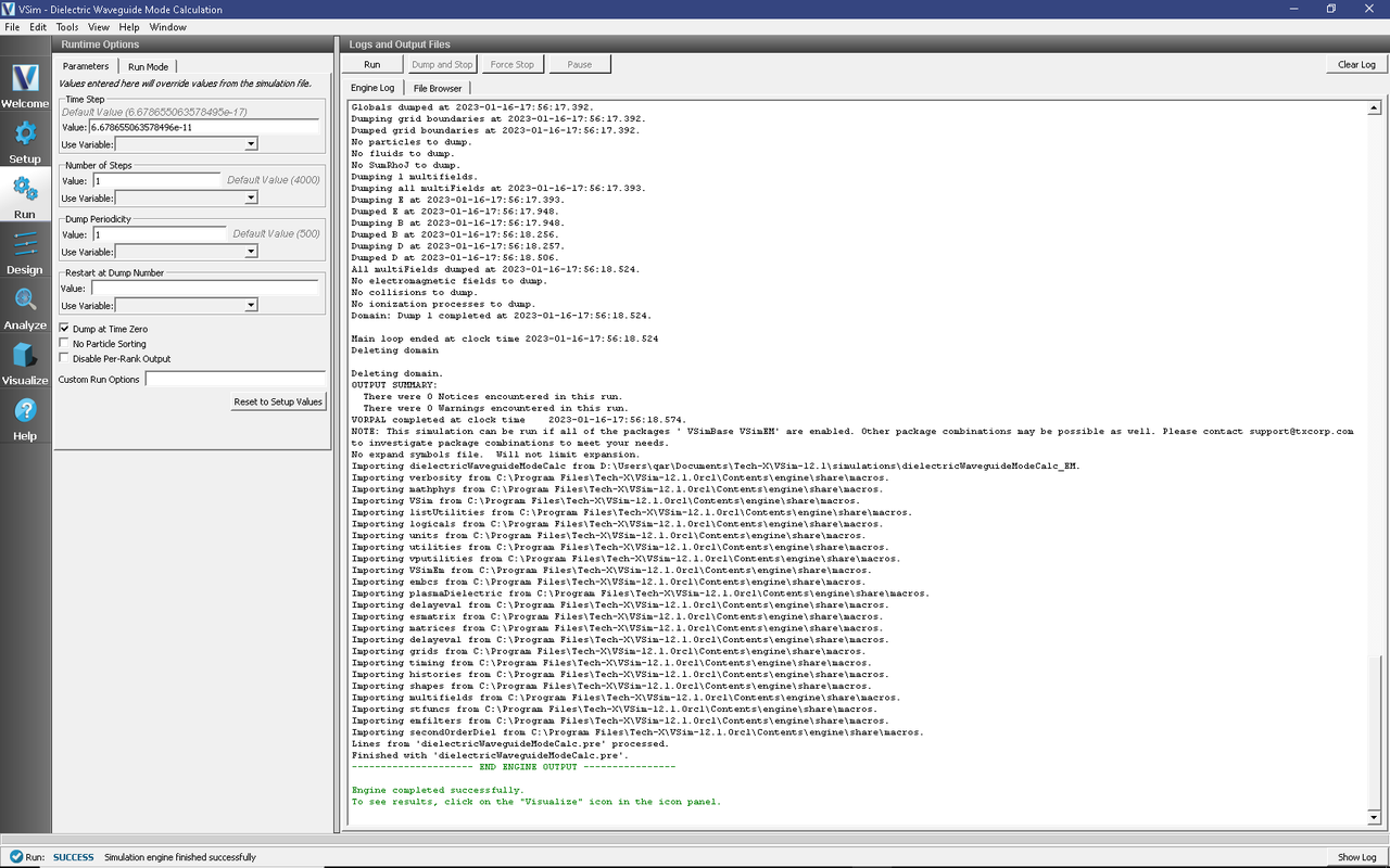
Fig. 271 Running the simulation for one step to get the permittivity data for the analyzer. Note that Dump at Time Zero is checked.
Solving for the Eigenmodes
After performing the above actions, continue as follows:
Proceed to the Analyze Window by clicking the Analyze button on the left.
Select computeWaveguideModes.py and click Open under the list.
Now update the analyzer fields accordingly. Some of these parameters are described above under Parameters
transverseSliceX 0.0
transverseSliceLY -0.7e-6
transverseSliceUY 0.7e-6
transverseSliceLZ -0.5e-6
transverseSliceUZ 0.5e-6
vacWavelength: 1.55e-6
nModes: 10
writeFieldProfile: H,E,D
We set the number of modes (nModes) to a value greater than the number of modes we expect. The analyzer will only find guided modes. Also check Overwrite Existing Files. Run the analyzer by clicking Analyze button in the upper right corner. The analyzer output should resemble Fig. 272. We see that the analyzer found 3 modes. They are listed in decreasing order of effective index.
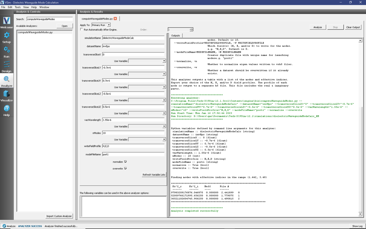
Fig. 272 The analyzer window after a successful run of computeWaveguideModes.py.
Visualizing the Results
After performing the above actions proceed to the Visualize window by pressing the Visualize button in the left column of buttons. You may need to Reload Data (bottom left). Visualize an eigenmode by following these steps:
From the Add a Data View dropdown, select Data Overview.
Expand Scalar Data, expand EigenD, and select EigenD_magnitude.
Below the visualization, the dump slider will allow you to scroll between the modes.
The resulting visualization pane should resemble Fig. 273.
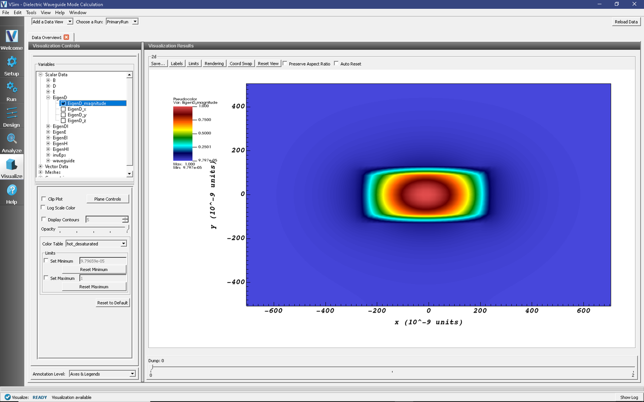
Fig. 273 The visualization pane showing the magnitude of the D field of the fundamental mode.
One can select other components of the H, E, or D field to see how they vary for the eigenmodes. These eigenmodes are now saved in .vsh5 files in the folder where the simulation was run.
Further Experiments
Change the geometry on the Setup window and rerun the simulation and analyzer to see the effects on the modes.
Once you have your desired mode, launch it down the waveguide using the procedure laid out in the multiModeFiberModeLaunchT example.
One can run a full convergence study of eigenmode effective indices by varying the RESOLUTION constant in the Setup window and re-running the simulation and mode extraction script. A plot of the effective index as a function of transverse cell area is shown in Fig. 274. The linear relationship shows the second order accuracy of our dielectric algorithms.
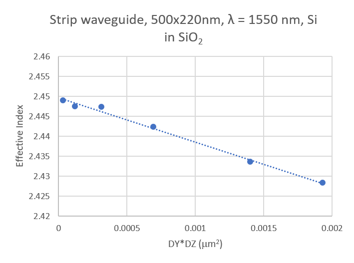
Fig. 274 The effective index as a function of transverse cell area for an eigenmode.