Kelvin-Helmholtz Instability (hydrodynamicImplosion.sdf)
Keywords:
- fluid, grid boundary, shock
Problem description
This example demonstrates the use of the Euler fluid solver to model a fluid shock reflecting around a square domain. This is based on the hydrodynamic implosion benchmark discussed in Liska, R., & Wendroff, B., “Comparison of Several difference schemes on 1D and 2D Test problems for the Euler equations.”
In this simulation, the density, flux, and energy density of a fluid are modeled via the Euler equations:
\(\frac{\partial n}{\partial t} = -\nabla \cdot (nv)\)
\(\frac{\partial nv}{\partial t} = -\nabla \cdot (nv \cdot v + Ip)\)
\(\frac{\partial nE}{\partial t} = -\nabla \cdot (vE)\)
The initial conditions of this simulation determine the evolving behavior. A step function in the density and pressure gives rise to a propagating shock wave that reflects off the sides of the box. After a long period the results can be compared to other simulation codes.
This simulation can be performed with a VSimBase license.
Opening the Simulation
The Hydrodynamic Implosion example is accessed from within VSimComposer by the following actions:
Select the New → From Example… menu item in the File menu.
In the resulting Examples window expand the VSim for Basic Physics option.
Expand the Basic Examples option.
Select “Kelvin-Helmholtz” and press the Choose button.
In the resulting dialog, create a New Folder if desired, and press the Save button to create a copy of this example.
All of the properties and values that create the simulation are now available
in the Setup Window as shown in hisetupwin.
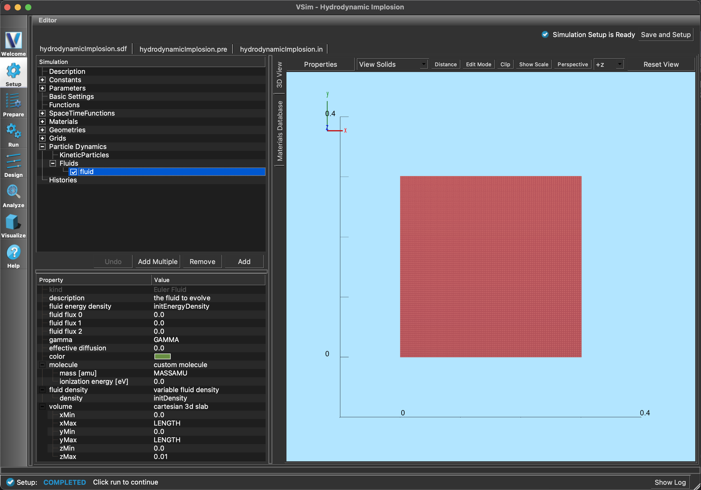
Setup Window for the Hydrodynamic Implosion example.
Simulation Properties
Constants are set up to allow setting the initial fluid conditions. The step function is defined by a low density (NLOW) and high density (NHIGH) along with a low pressure (PLOW) and high pressure (PHIGH). The gas gamma (GAMMA) is set to 1.4, and the length of the box that constrains the fluid (BOXLENGTH) is 0.3. Finally, the density/pressure step function is set to exist as x + y = 0.15.
Running the Simulation
After performing the above actions, continue as follows:
Proceed to the Run Window by pressing the Run button in the left column of buttons.
To run the file, click on the Run button in the upper left corner of the
Logs and Output Files* pane. You will see the output of the run in the right pane. The run has completed when you see the output, “Engine completed successfully.” A snapshot of the simulation run completion is shown in
hirunwin.

The Run Window at the end of execution.
Visualizing the Results
The density shown in hivizwin shows the final density contours at
time t=2.5. A msuhroom shape structure of low density remains in the lower
left corner of the domain, and a low density jet has shot out along the
diagonal due to the repeated impact of the reflecting shocks. These results
are consistent with the benchmark reuslts in the paper, though the diagonal
fluid jet is less well-defined, indicating a larger amount of numerical
dissipation than some other methods/codes.

The fluid density.