A6 Magnetron 2: Power (a6Magnetron2Power.sdf)
Keywords:
- magnetron, bunching, space charge, A6
Warning
Due to the randomness of the particle generation, the results of this example will differ slightly with MPI ranks. To reproduce the images exactly described in this documentation, we recommend using an MPI setting of 4 cores.
Problem Description
This VSimVE example simulates MIT’s cylindrical A6 magnetron cavity with a slot outlet in three dimensions. The geometry was defined by using VSimComposer’s constructive solid geometry (CSG) capabilities. The cathode-anode voltage is ramped up from zero to around \(360~\mathrm{kV}\) by a current distribution source. Electrons are emitted from the emitter section of the cathode, and undergo \(E\times B\) drift. Bunching of the space-charge distribution occurs and kinetic energy from the electrons is transferred to the electromagnetic modes of the cavity. If the simulation is run long enough, it will be seen that the \(2\pi\) mode dominates.
This simulation can be performed with a VSimVE license.
Opening the Simulation
The A6 Magnetron example is accessed from within VSimComposer by the following actions:
Select the New → From Example… menu item in the File menu.
In the resulting Examples window expand the VSim for Vacuum Electronics option.
Expand the Radiation Generation option.
Select A6 Magnetron 2: Power and press the Choose button.
In the resulting dialog, create a New Folder if desired, and press the Save button to create a copy of this example.
All of the properties and values that create the simulation are now
available in the Setup Window as shown in
Fig. 396. You can expand the tree elements and
navigate through the various properties, making any changes you
desire. The right pane shows a 3D view of the geometry, if any, as
well as the grid, if actively shown. To show or hide the grid, expand
the Grid element and select or de-select the box next to Grid.
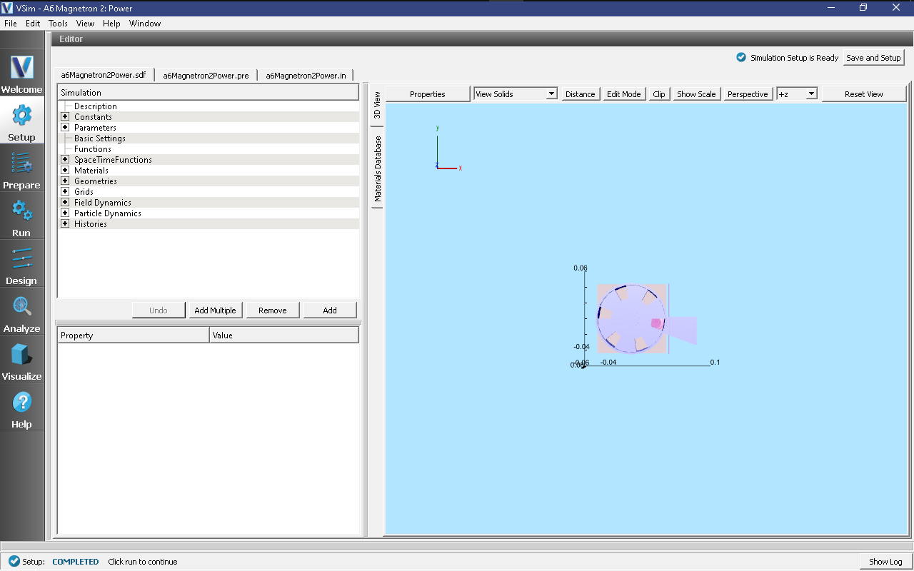
Fig. 396 Setup Window for the A6 Magnetron example.
Simulation Properties
The A6 Magnetron example includes several constants for easy adjustment of simulation properties. User changeable parameters include:
RADIUS_ANODE → Inner radius of anode.
RADIUS_ANODE_OUTER → Outer radius of anode.
ANGLE_CAVITY → Angle of resonant cavity openings, in degrees.
THICKNESS_WALL_OUTER → Thickness of all walls.
WIDTH_MAGNETRON → Total width of magnetron in z-direction.
RADIUS_OUTLET → Radius of outlet horn in x-direction.
WIDTH_IRIS → Width of outlet slit opening.
WIDTH_VANES → Total width of anode vanes in z-direction.
RADIUS_CATHODE → Radius of the emitting section of the cathode.
RADIUS_CATHODE_INNER → Radius of the inner section of the cathode.
WIDTH_CATHODE → Width (in z-direction) of the emitting section of the cathode.
(X,Y,Z)POS_HIST → Position of electric field history.
The axial magnetic field is uniform with a constant value of \(B_{z}=0.6~\mathrm{T}\). There is an opening at the back of one of the cavities that allows microwave energy to leave the magnetron through a horn antenna and into a matched absorbing layer (MAL) boundary. A Poynting Flux history records the power output through the antenna. The emitting region of the cathode has a slightly larger radius than the rest of the cathode. There are also end caps, on either side of the vanes, in electrical contact with the cathode.
Running the Simulation
After performing the above actions, continue as follows:
Proceed to the Run Window by pressing the Run button in the left column of buttons.
Here you can set run parameters, including how many cores to run with (under the MPI tab).
When you are finished setting run parameters, click on the Run button in the upper left corner. You will see the output of the run in the right pane. The run has completed when you see the output, “Engine completed successfully.”
This simulation is setup so that the cathode emission current and anode-cathode (AK) voltage ramp up relatively slowly (over many RF periods). Once the AK voltage is high enough, the bunching of the electrons will occur. If the simulation is run for long enough, around 100000 time steps, the \(2\pi\) mode will eventually dominate as has been seen experimentally for this magnetron.
Visualizing the results
After performing the above actions, continue as follows:
Proceed to the Visualize Window by pressing the Visualize button in the left column of buttons.
After the simulation has been run for a sufficient amount of time, spokes will form in the electron distribution (bunching). Since the A6 is a six-cavity magnetron, operation in the \(2\pi\) mode will correspond to six spokes. To visualize the spokes:
Select Phase Space from the Data View pull-down menu
Select electrons_x for the X-axis
Select electrons_y for the Y-axis
Use the Dump bar at the bottom of the screen to advance through the solution and visualize each dump file
Eventually, a steady state will be reached in which the electron distribution has six spokes similar to Fig. 397 taken at Dump 35.
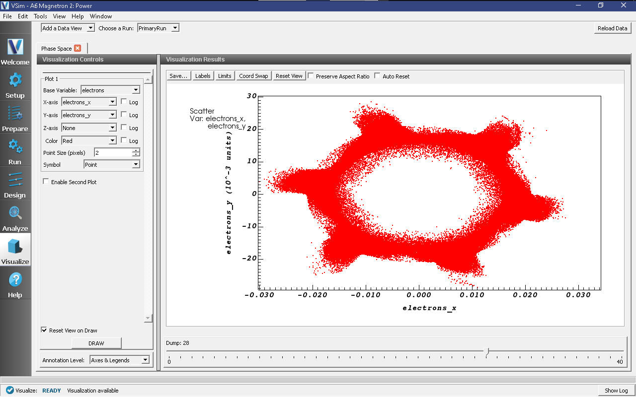
Fig. 397 Phase-space plot of the electron distribution showing the formation of six spokes corresponding to operation in the \(2\pi\) mode.
To visualize the axial magnetic field during the \(2\pi\) mode operation, proceed as follows:
Select Data Overview from the Data View pull-down menu
Expand B
Select B_z
Select the Clip Plot checkbox
Check the Set Minimum box and set the value to -0.06
Check the Set Maximum box and set the value to 0.06
Expand Geometries
Select poly (a6Magnetron2PowerPecShapes)
Select the Clip Plot checkbox
Move the dump slider forward in time to see the evolution.
Image Fig. 398 was taken at Dump 35.
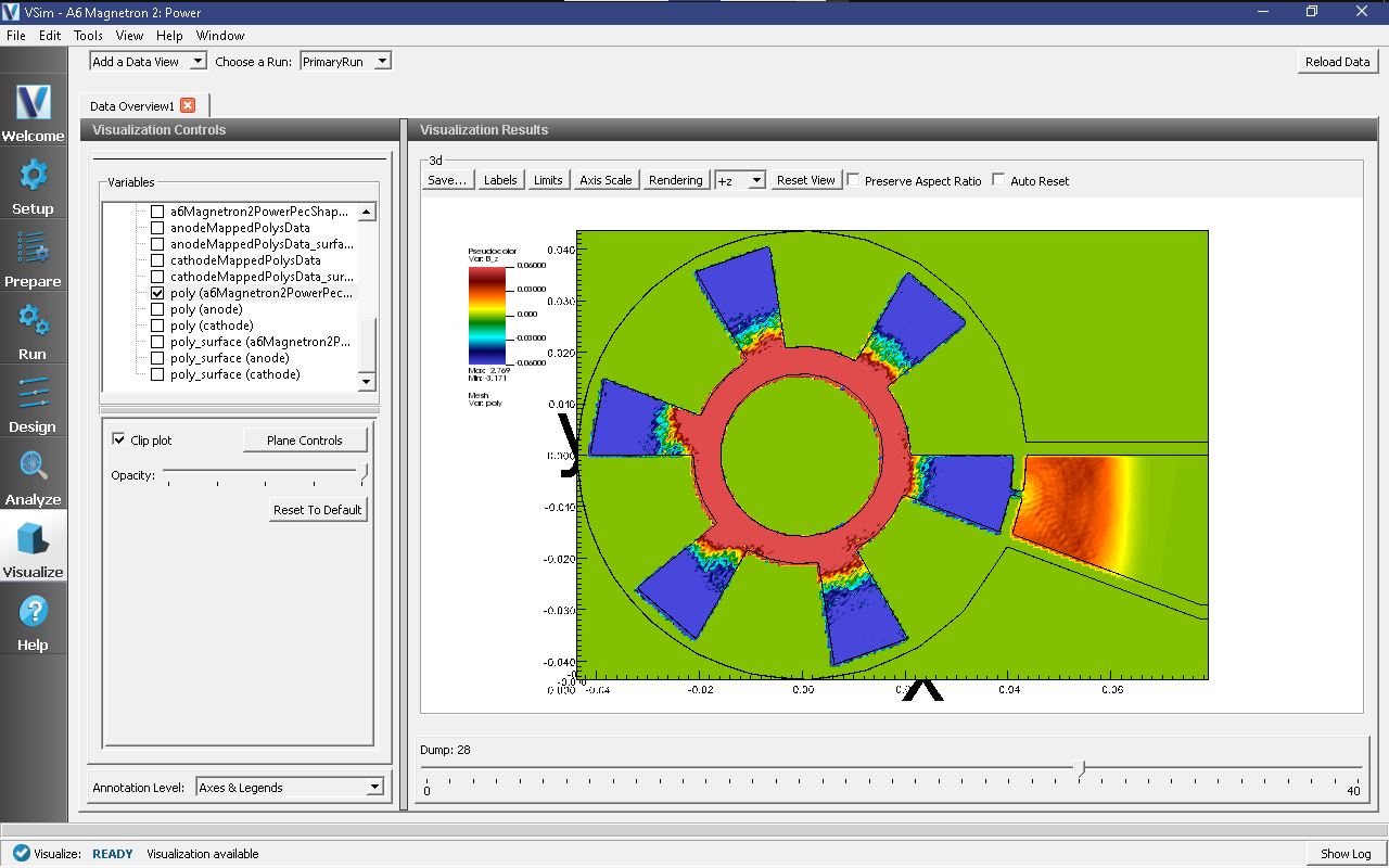
Fig. 398 Axial magnetic field of the magnetron operating in the \(2\pi\) mode.
To determine the operating frequency:
Select History from the Data View pull-down menu
Select outB_2 for Graph 1 and Graph 2
Click Fourier Amplitudes (dB) to the left of one of the plots in the Visualization Results pane
Zoom in on the maximum of this plot to determine the approximate resonance mode frequencies
The resulting plot will resemble Fig. 399. If the simulation has been run for long enough, the peak at \(4.6~\mathrm{GHz}\), which corresponds to the \(2\pi\) mode, should be the most prominent.
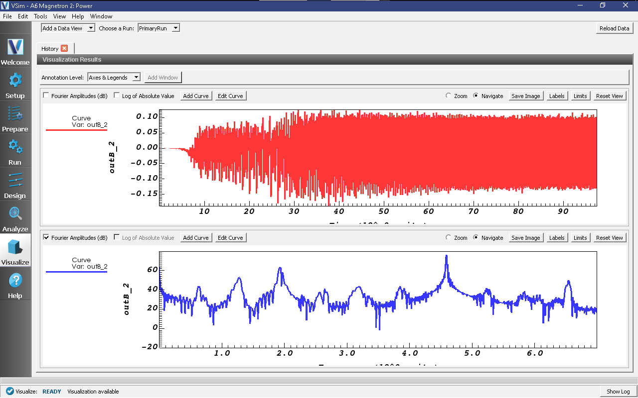
Fig. 399 Plot of outB_2 vs. time and vs. frequency (Fourier transform).
Further Experiments
The power output and operating mode is affected by the \(E/B\) ratio and the geometry. The user could try adjusting the strength of the magnetic field and the geometry of the cathode, including the radius of the emitting region and the configuration of the end-caps, to see how this affects magnetron operation.