Penning High Intensity Ion Source (PenningSource.sdf)

Keywords:

coherent ion beam, electron emitters, electron-neutral collisions, plasma source

Problem Description

This Penning Source example illustrates how to generate an electron population by emitting electrons off of a cathode using VSim’s Settable Flux Shape Emitter model. The charge neutral plasma forms due to impact ionization from electron-neutral collisions which ionizes the neutral Argon gas to generate a second electron (in each collision) and a singly charged Argon ion. This simulation also includes impact excitation and elastic collisions between electrons and Argon gas. The various types of elastic and inelastic collisions of the particles are calculated with the Vorpal engine’s Monte Carlo package. The plasma particles, background gas, and collisions are set up in the Particle Dynamics Element. The cross-sections for these collisions are imported from 2-column data files. The electrons are attracted in to the plasma chamber by charging the anode (filled with Argon gas) to a positive potential. Secondary electrons are emitted off the anode due to the primary electrons interacting with the anode walls. This is set up using a Secondary Emitter model in VSim.

The Argon ions are then extracted from the plasma source with two extraction plates biased to a large negative potential. The two extraction plates accelerate the ions out of the plasma generating an ion beam which is focused to a small width according to the space between the two extraction plates. To further focus the ion beam, absorbing plates are placed below the extraction plates which are part of the anode. A 0.16 Tesla magnetic field in the \(y-\textrm{direction}\) is imposed to restrict the motion of the electrons in the Anode region. For the example shown here a Space Time Function is used to confine the magnetic field to a specified region using a Heaviside Step function. The electric field is solved via Poisson’s equation using a Generalized Minimal Residual (GMRES) linear solver. This solver is chosen under Field Dynamics -> PoissonSolver. A combination of Dirichlet and Neumann boundary conditions involving the shapes and simulation boundaries are imposed. Field boundary conditions are imposed under Field Dynamics -> FieldBoundaryConditions. The plasma is represented by macro-particles which are moved using the Boris scheme in a 3D Cartesian coordinate system.

This simulation can be run with a VSimPD license.

Opening the Simulation

The Penning Source example is accessed from within VSimComposer by the following actions:

• Select the New → From Example… menu item in the File menu.

• In the resulting Examples window expand the VSim for Plasma Discharges option.

• Expand the Ion Sources option.

• Select Penning High Intensity Ion Source and press the Choose button.

• In the resulting dialog, create a New Folder if desired, then press the Save button to create a copy of this example.

All of the properties and values that create the simulation are now available in the Setup Window as shown in Fig. 518. You can expand the tree elements and navigate through the various properties, making any changes you desire. Please note that many options are available by double clicking on an option and also right clicking on an option. The right pane shows a 3D view of the geometry as well as the grid. To show or hide the grid, expand the “Grid” element and select or deselect the box next to Grid. You can also show or hide the different geometries by expanding the “Geometries” element and selecting or deselecting “anodePlasmaPlate”, “cathode” and/or “extractionPlates”. Note that these three shapes are unions of the other more basic shapes included in this simulation.

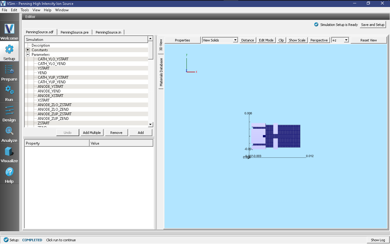
Fig. 518 Setup window for the Penning Source example.

Simulation Properties

This example contains many user defined Constants which help simplify the setup and make it easier to modify. The following constants can be modified by left clicking on Setup on the left-most pane in VSim. Then left click on + sign next to Constants and all the constants used in the simulation will be displayed. To add your own constant, right click on Constants and left click on Add User Defined. Below is an explanation of a few of the constants used. There are several more constants included in the simulation.

XSTART/XEND,YSTART/YEND,ZSTART/ZEND: Physical dimensions of simulation in meters.

CATHODE_VOLTAGE: Potential of electron source from which electrons are emitted

ANODE_VOLTAGE: Potential of anode which attracts the electrons from the cathode

PENNING_MAGNETIC_FIELD: Magnetic of external magnetic field used to confine the ion beam

T1: Time that the electrons are emitted from the electron source.

Running the Simulation

Once finished with the setup, continue as follows:

• Proceed to the Run Window by pressing the Run button in the navigation column out left.

• To run the file, click on the Run button in the upper left corner of the Logs and Output Files pane.

You will see the output of the run in that pane. The simulation takes about 1500 time steps before an ion beam is observed to begin forming and 4000 time steps before a persistent modestly dense beam has formed. The run has completed successfully when you see the output, “Engine completed successfully.” This is shown in Fig. 519.

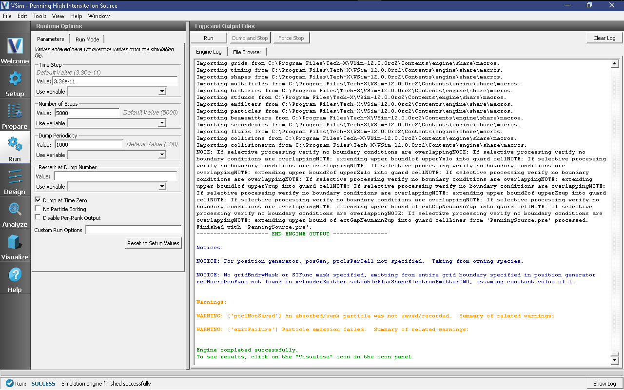
Fig. 519 The Run Window at the end of execution.

Analyzing the Results

After performing the above actions, continue as follows:

• Proceed to the Analysis Window by pressing the Analyze button in the navigation column.

• In the resulting list of Available Analyzers, select computePtclNumDensity.py and press Open

• The analyzer fields should be filled as below:

  • simulationName: penningSource

  • speciesName with “electrons” or “Ar1” which are the names of the two species in the “Particle Dynamics” tab in the visual setup.

• Click Analyze in the top right corner.

• The analysis is completed when you see the output shown in Fig. 520.

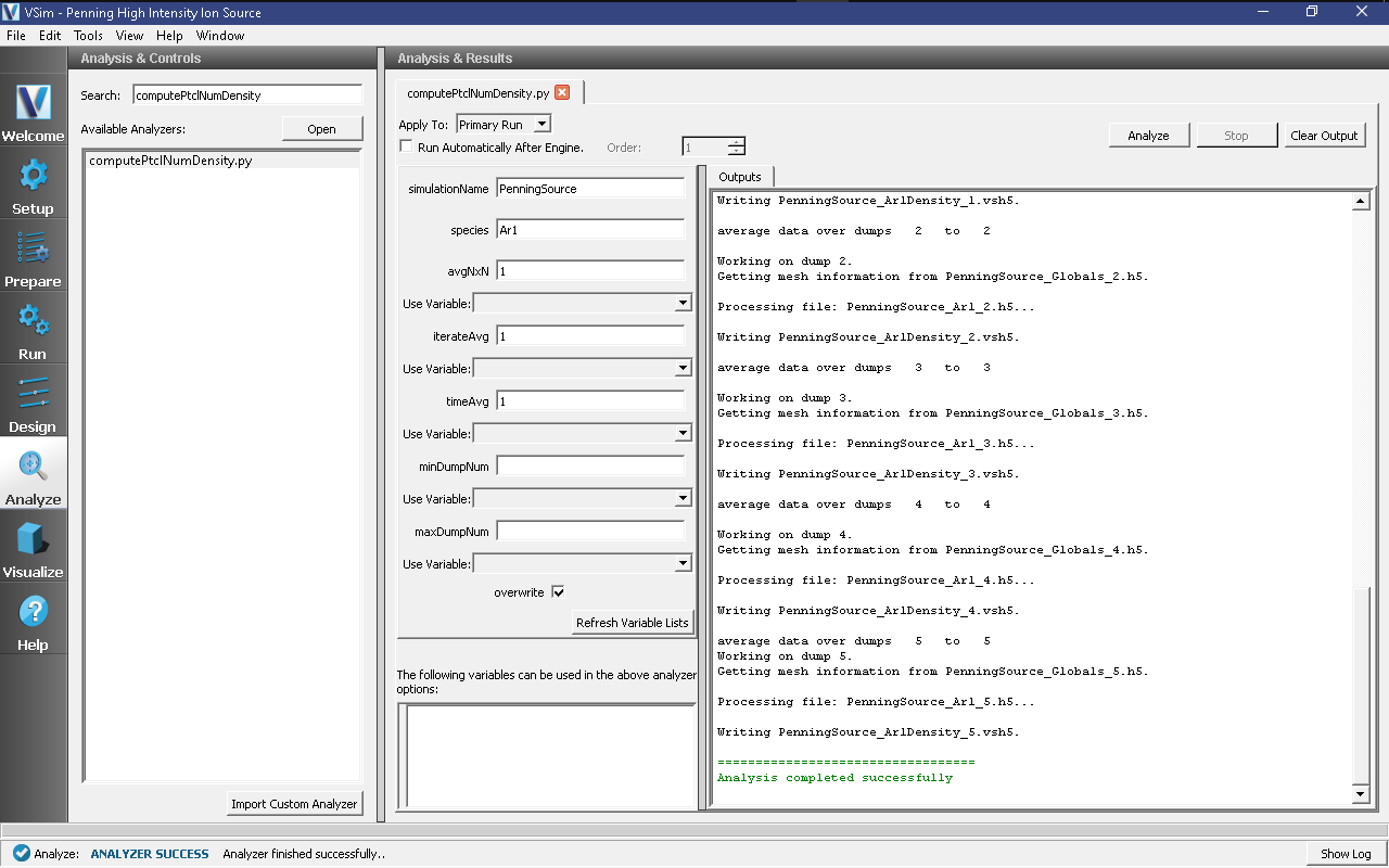
Fig. 520 The Analyze Window at the end of a successful run.

The resulting data is called electronDensity and Ar1Density and shows the number density in the 3D simulation domain in units of #/m^3.

Visualizing the Results

After performing the above actions, the results can be visualized as follows:

• Proceed to the Visualize Window by pressing the Visualize button in the navigation column.

• Clicking on the Add a Data View dropdown menu shows there are many different types of data to visualize.

• To get started, lets visualize the formation of the plasma in the anode and the resulting ion beam.

• Click on the Data Overview tab which is a default tab already loaded in the “Visualize” section of VSim.

• Under Variables, click on “Particle Data”, “electrons” and the top most box (“electrons”)

• Click on “Ar1” then click on the top most box (“Ar1”)

• Finally, to visualize the plasma species in the context of the geometries in the simulation, click on “Geometries”, “poly(cathode)”, “poly(extractionPlates)”, and “poly(anodePlasmaPlate)”.

• You can rotate the figure by holding down the left mouse button and moving the mouse.

• Slide the bar to the right at the bottom of the display window to watch the ions form and accelerate out of the anode.

The resulting visualization is shown in Fig. 521.

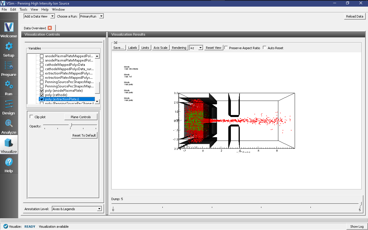
Fig. 521 The evolved ion beam near the end of the simulation.

This plot shows that the ions have been extracted from the plasma reservoir to form a coherent ion beam.

Next you can visualize phase space which is a plot of velocity vs distance. Click on “Add a Data View” at the top left of the Visualization window. Then click on “Phase Space”. A visualization tab will open next to “Data Overview”. Next to “Base Variable”, click “Ar1”. For the “X-axis”, choose Ar1_x and for the “Y-axis”, choose Ar1_ux. This produces a plot of velocity vs. position. Finally, you can include position along the z-axis by clicking on the “Color” tab and choosing Ar1_z and clicking “DRAW” at the bottom of the screen. The color indicates the location along the z-axis of each particle.

The visualization window showing phase space is shown in Fig. 522.

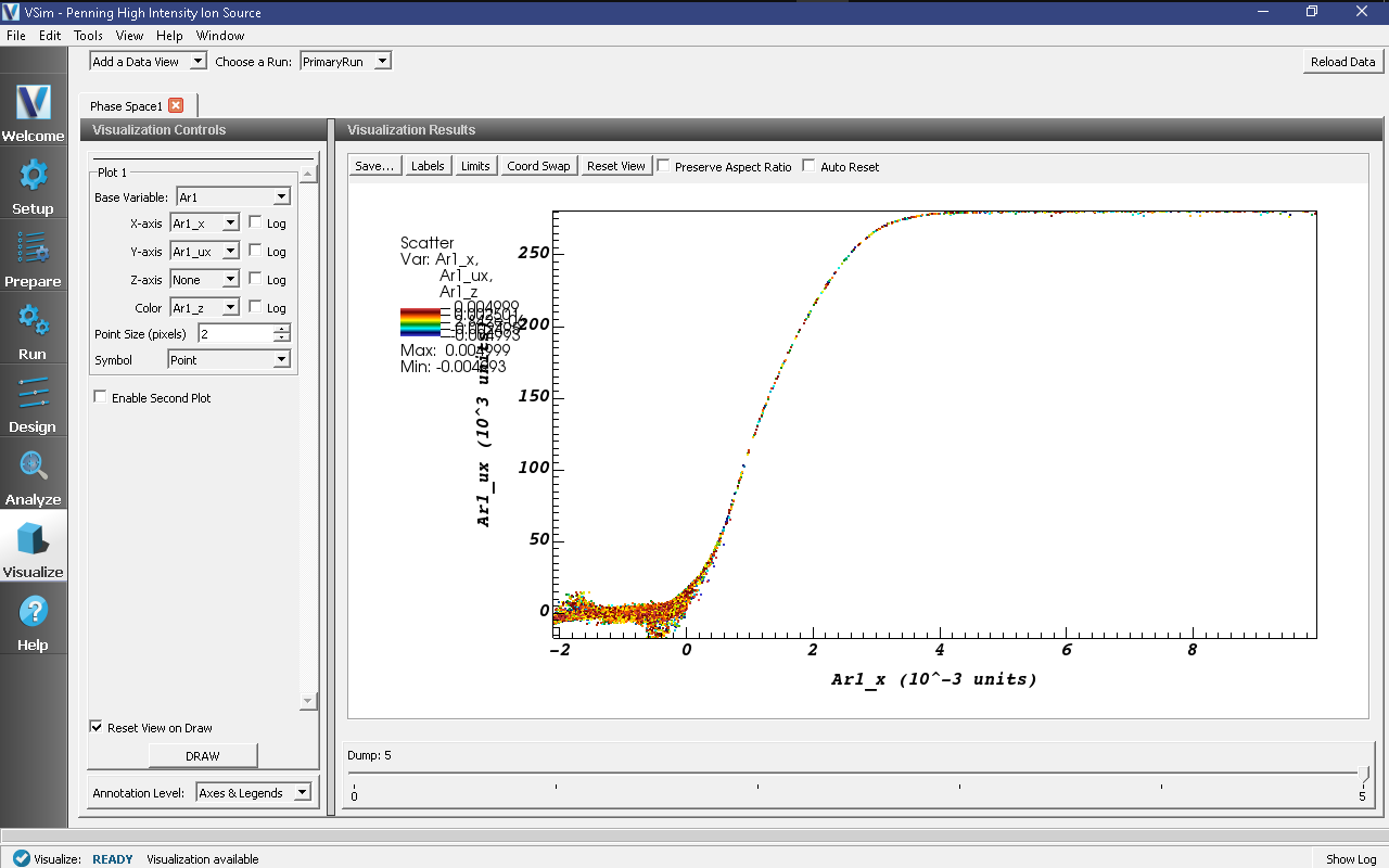
Fig. 522 Plot of phase space (vx vs x).

Further Experiments

For this simulation, sample cross sections were used which are not necessarily the correct ones. The VSim interface can import any cross sections that are in a 2-column format. There should be NO headings in the data file. The LXcat scattering database (https://fr.lxcat.net/data/set_type.php) and EEDL cross section database contain cross section data for around one hundred different materials. As another experiment, change the cross-section used in the simulation or change the species of the background gas and import new cross-sections.

Set up a History that records the Ar1 current flowing out of the plasma chamber on to the x=XEND boundary. Right click on the “Histories” element and under “Add ParticleHistory” select “Absorbed Particle Current.” You can change the name of the history by double clicking on the new “absorbedPtclCurrent0” element in the tree. Then be sure to pick the particle absorber from which you would like to collect data. Note that to add a history on a boundary, that boundary needs to be of type “Absorb and Save”.

The Reactions framework allows one to set up collision interactions flexibly. The collisions involved in this example are electron-neutral collisions that lead to ionization and ohmic heating. As a further experiment, ion-neutral collisions, such as elastic scattering and charge exchange, can also be added to the simulation.