Single Particle Circular Motion (singleParticleCircularMotion.sdf)
Keywords:
- single particle, circular motion, finite difference effects
Problem Description
This example shows how to simulate the uniform circular motion of a single electron in a constant, uniform magnetic field in VSim. The electron is loaded inside a cylindrical capacitor with grounded walls to eliminate any stray electric fields. The electron is loaded far from the walls to reduce any effects from image charges. The magnetic field points down the positive z-axis.
Due to the finite difference algorithm utilized by VSim, two corrections must be made in order to get the electron to take a true circular trajectory. The first correction is to the cyclotron frequency. In the finite difference world of VSim, the electron does not move along a circular arc from time step to time step, instead it moves along a straight line. To correct for this we need to set our \(\omega_{cyclo_{FD}} = \frac{2}{\Delta T} \arctan \left( \frac{\omega_{cyclo} \Delta T}{2} \right)\) [1] (see chapter 4 section 3).
The next correction is to account for the implementation of the Boris Method [1], the algorithm used in VSim to push particles. In the Boris Method, the position of the particle, \(\vec{x}(t)\), is defined at full time steps, while the velocity, \(\vec{v}(t)\), is defined at half time steps. This scheme of ‘well-centered’ derivatives means that VSim is automatically accurate to second order, but it means we have to be careful about our initial conditions for the electron’s velocity. The initial velocity is set under Particle Dynamics → Kinetic Particle → electrons0 → particleLoader0 then velocity distribution. VSim will assume that this is the particle’s velocity a ONE HALF time step before the start of the simulation, so we must load the particle with the velocity it would have a half time step before the start of the simulation.
This simulation can be performed with a VSimBase license.
Opening the Simulation
The Single Particle Circular Motion example is accessed from within VSimComposer by the following actions:
Select the New → From Example… menu item in the File menu.
In the resulting Examples window expand the VSim for Plasma Discharges option.
Expand the Processes option.
Select Single Particle Circular Motion and press the Choose button.
In the resulting dialog, create a New Folder if desired, and press the Save button to create a copy of this example.
All of the properties and values that create the simulation are
now available in the Setup Window as shown in
Fig. 579.
You can expand the tree elements and navigate through the various
properties, making any changes you desire. The right pane shows
a 3D view of the geometry, if any, as well as the grid, if
actively shown. To show or hide the grid, expand the Grid
element and select or deselect the box next to Grid.
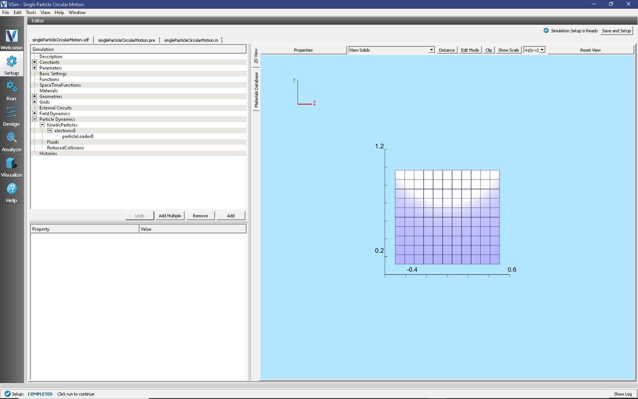
Fig. 579 Setup Window for the Single Particle Circular Motion example.
Simulation Properties
The Single Particle Circular Motion example includes some constants for easy adjustment of simulation properties:
B0: The magnitude of the magnetic field
VOLTAGE_OUTER and VOLTAGE_INNER: sets the value of the radial electric field experienced by electron (default value for both is zero)
Running the Simulation
After performing the above actions, continue as follows:
Proceed to the Run Window by pressing the Run button in the left column of buttons.
Here you can set run parameters. The default is to run in serial.
To run the file, click on the Run button in the upper left corner of the Logs and Output Files pane. You will see the output of the run in this pane. The run has completed when you see the output, “Engine completed successfully.” This is shown in Fig. 580
In serial, this simulation only takes seconds to run.
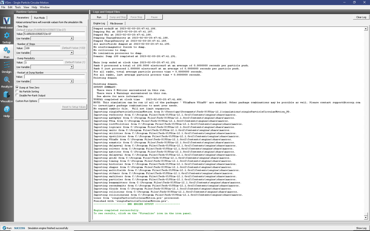
Fig. 580 The Run Window at the end of execution in serial.
Visualizing the results
After performing the above actions, continue as follows:
Proceed to the Visualize Window by pressing the Visualize button in the left column of buttons.
In the Visualize Window, expand ‘Particle Data’ then ‘electrons0’ and check the box next to the red ‘electrons0.’ This will plot our single electron.
Expand ‘Meshes’ then ‘globalGridGlobal’ and check the box next to ‘globalGridGlobal (ChargeDensity)’ as shown in Fig. 581.
Scroll through the dump slider (found below the plot), the electron will be stationary because the axial coordinate (\(phi\)) has been compressed. This means the electron remains at the same r and z coordinate (this is a 2D simulation).
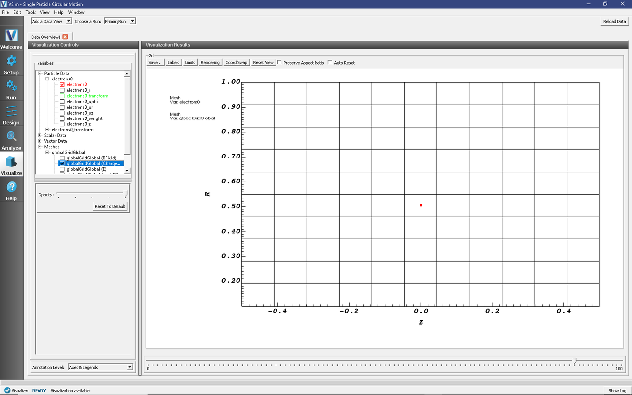
Fig. 581 Visualization of Single Particle Circular Motion at dump 100.
Further Experiments
Simulations are correct only to some accuracy. The corrections we made to the cyclotron frequency and the initial velocity make this simulation correct to second order. By looking at the phase space plot, we can explore the second order accuracy of this simulation. Navigate to the Visualize Window, select ‘Phase Space’ from the ‘Data View’ drop down menu, and plot ‘electrons0_r’ vs ‘electrons0_ur.’
As you scroll through the dumps for the first time (with the ‘Auto Reset’ box UN-checked), the axes will adjust. The particle is taking an elliptical path in phase space. In a perfect simulation, the electron would remain at the same position in phase space with constant radius and zero radial velocity. Instead, the electron oscillates between the positions \(r = 0.50500\) m and \(r = 0.50542\) m for a \(\Delta r = 0.00042\) m. Cut the time step in half and double the number of timesteps taken (so that the simulation runs through the same amount of time). Now look at the phase space plot again. By approximately what factor did \(\Delta r\) drop? Since the simulation is correct to second order, dropping the time step by a factor of 2 should drop the error by a factor of 4.
Other things you can play around with:
Reset the electron speed, electron loading position, or the cyclotron frequency, OMEGA, back to the uncorrected versions and redo the error analysis described above.
Change the values for VOLTAGE_INNER and VOLTAGE_OUTER to see the effects of a radial electric field on the single electron.
References
[1] Birdsall, C. K., & Langdon, A. B. (1985). Plasma Physics via Computer Simulation. New York: McGraw-Hill.