Proton Beam (protonBeam.sdf)

Keywords:

electromagnetic, particle in cell, material boundary, reactions, particle emitter

Problem description

This example injects a proton beam into a column of neutral H2 gas. The geometry is setup like an electron column in an accelerator beamline (i.e. external solenoidal B-field and negative electrodes on either end for electron confinement). Upon entering the neutral gas multiple reactions begin to occur including ionization, charge exchange, dissociation, H3+ formation, and others. The beam leaves the column, leaving behind a combination of ions, electrons, and neutrals that are either confined or ejected by the background electrode potential.

In this simulation, a beam of H+ ions propagates through a background H2 gas. Collisions between the beam ions and the background gas produce electrons, H2+, neutral H, and H3+ through the following reactions:

\(H^+ + H_{2} \rightarrow H^+ + H_{2}^+ + e^-\) (ion impact ionization)

\(e^- + H_{2} \rightarrow H_{2} ^+ + 2e^-\) (electron impact ionization)

\(H^+ + H_{2} \rightarrow H^+ + H_{2}\) (elastic)

\(H^+ + H_2 \rightarrow H + H_2^+\) (charge exchange)

\(H_2^+ + H_2 \rightarrow H_3^+ + H\) (H3+ formation)

\(H_2^+ + H_2 \rightarrow H_2^+ + H_2\) (charge exchange)

\(H_2 + e^- \rightarrow H^+ + H + 2e^-\) (dissociative ionization)

\(H_3^+ + H_2 \rightarrow H_3^+ + H_2\) (elastic)

Fig. 574 shows the cross sections for the above reactions as a function of incident energy.

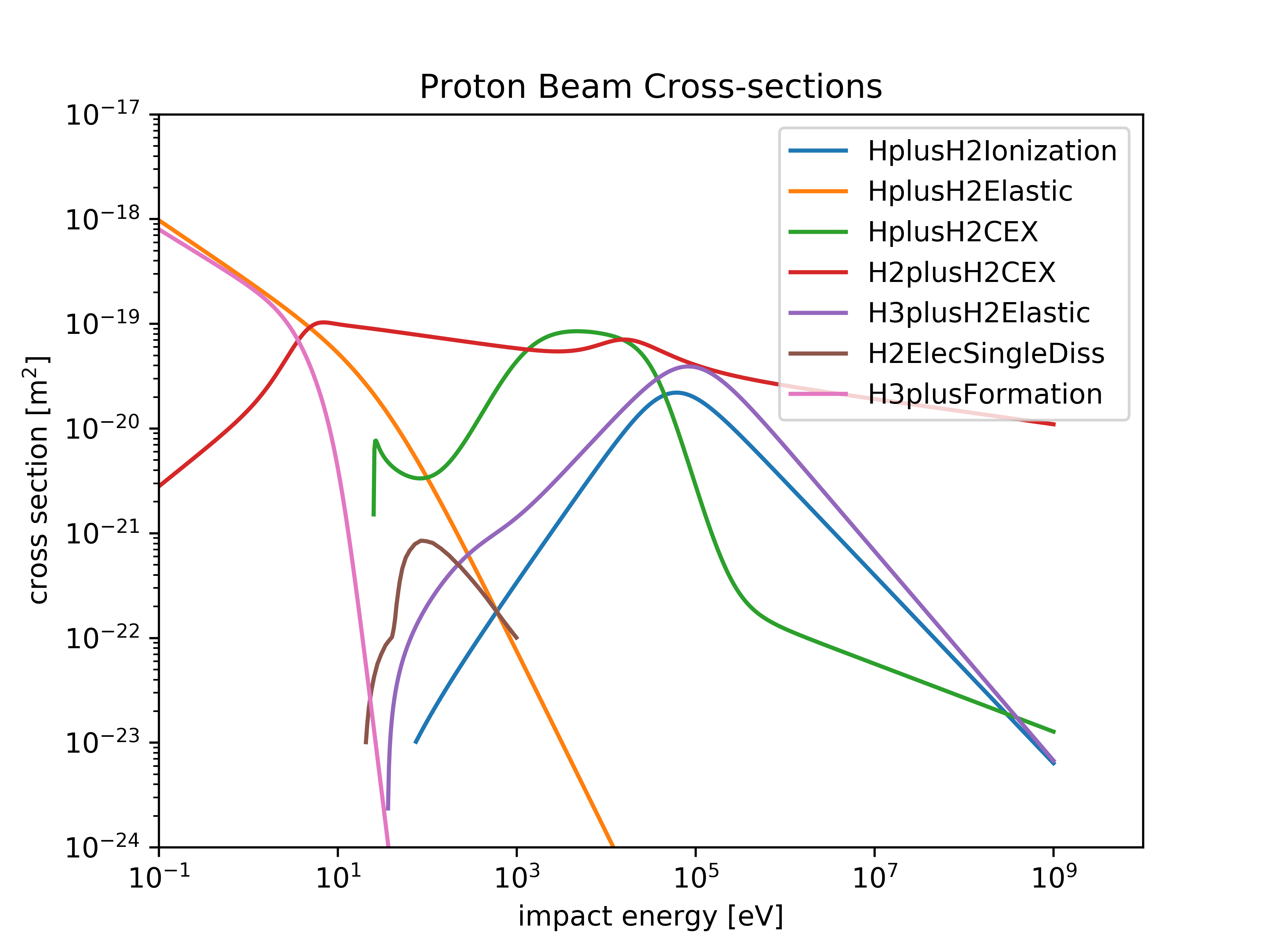
Fig. 574 Cross sections for the collisions included in this example.

This simulation can be performed with a VSimPD license.

Opening the Simulation

The Proton Beam example is accessed from within VSimComposer by the following actions:

• Select the New → From Example… menu item in the File menu.

• In the resulting Examples window expand the VSim for Plasma Discharges option.

• Expand the Processes option.

• Select “Proton Beam” and press the Choose button.

• In the resulting dialog, create a New Folder if desired, and press the Save button to create a copy of this example.

All of the properties and values that create the simulation are now available in the Setup Window as shown in Fig. 575. You can expand the tree elements and navigate through the various properties, making any changes you desire. The right pane shows a 3D view of the geometry, if any, as well as the grid, if actively shown. To show or hide the grid, expand the Grid element and select or deselect the box next to Grid.

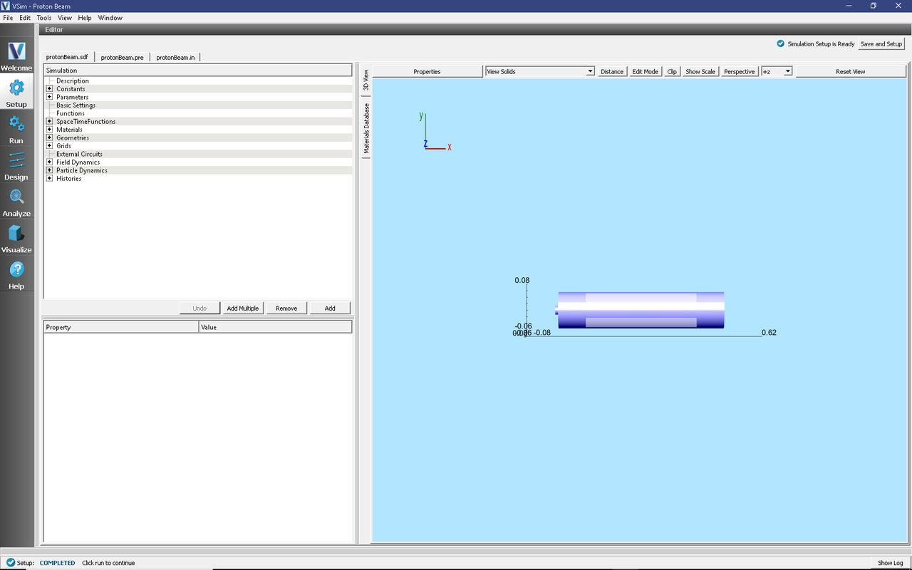
Fig. 575 Setup Window for the Proton Beam example.

Simulation Properties

Constants are set up to allow setting the proton beam energy and current, the background H2 pressure and temperature, and the cross-sectional size of the beam emission.

Running the Simulation

After performing the above actions, continue as follows:

• Proceed to the Run Window by pressing the Run button in the left column of buttons.

• To run the file, click on the Run button in the upper left corner of the Logs and Output Files pane. You will see the output of the run in the right pane. The run has completed when you see the output, “Engine completed successfully.” A snapshot of the simulation run completion is shown in Fig. 576.

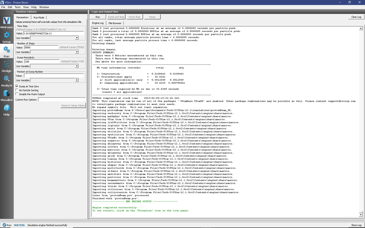
Fig. 576 The Run Window at the end of execution.

Visualizing the Results

We can now visualize all of the particles at a particular time slice. To do this:

• Proceed to the Visualize Window by pressing the Visualize button in the left column of buttons

• Expand Particle Data and select Electrons, H2Plus, and Hplus.

• Slide the time slider to advance the simulation in time (step 50 is shown in Fig. 577)

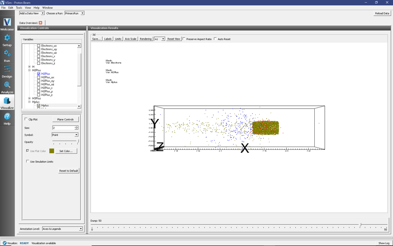
Fig. 577 Plot of all the particles at timestep 50. Notice that the electrons are confined by the magnetic field to the inner radius of the device. Some will also be confined by the electrodes to oscillate along the device.

Next we can visualize the potential due to the particles and the electrodes:

• Unselect the particle data (Electrons, H2Plus, and Hplus).

• Expand Scalar Data and select Phi.

• Check the Clip All Plots box and scroll through the dumps.

The potential shown in Fig. 578 is the total potential, that is, the potential due to the static electrodes, the proton beam, and other charged species resulting from the reactions.

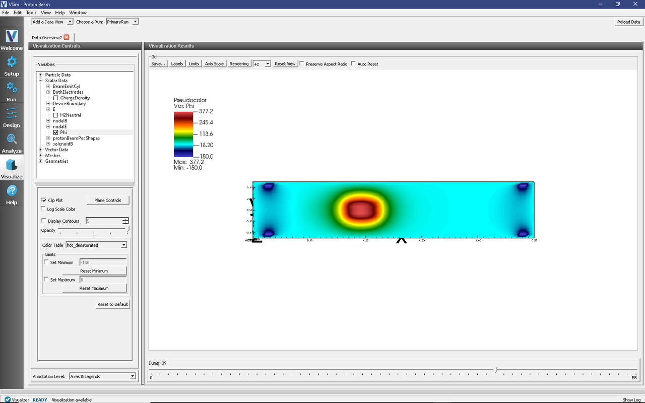
Fig. 578 The electrostatic potential

Further Experiments

Try changing the neutral gas pressure (which in turn will modify its density). At higher densities more reactions will occur and the proton beam will not be able to traverse the column intact. For lower densities, which are more in line with experiment, the proton beam will cause small amounts of ionization in the background gas, generating an electron cloud that is confined by the electrodes that can provide space-charge compensation for the beam. Lowering the beam energy will allow some lower energy reactions, such as H3+ formation, to occur.