Neutral Heat Transport DSMC (neutralHeatTransport.sdf)
Keywords:
- heat transport, DSMC, elastic collisions, reactions
Problem description
VSim may be used to model the heat flux through a neutral gas confined between two plates of different temperatures. This problem is a common benchmark for DSMC simulations, and is described by Bird in “Molecular gas dynamics and the direct simulation of molecular gas flows” (1994) on page 280. In this example, we model the heat transport between cold (250K) and hot (1000K) plates separated by a meter. Between the plates is a volume of neutral Argon gas that transports the heat through either free-molecular motion (in the case of lower pressure) or through collisional transport via elastic collisions (in the case of higher pressure). The simulated heat flux can then be compared to the analytic result, validating the reactions framework in VSim.
This simulation can be performed with a VSimPD license.
Two videos are available demonstrating this example: https://www.youtube.com/watch?v=FFgqtJASseM&list=PLottQ0Bg2M-3ATV5O9IP-3TEC4toVYPAK&index=8 https://www.youtube.com/watch?v=WWbQ6uq1LOo&list=PLottQ0Bg2M-3ATV5O9IP-3TEC4toVYPAK&index=7
Opening the Simulation
The Neutral Heat Transport example is accessed from within VSimComposer by the following actions:
Select the New –> From Example… menu item in the File menu.
In the resulting Examples window expand the VSim for Plasma Discharges option.
Expand the Processes option.
Select “Neutral Heat Transport” and press the Choose button.
In the resulting dialog, create a New Folder if desired, and press the Save button to create a copy of this example.
The Setup Window is shown with all the implemented physics and geometries in Fig. 570.
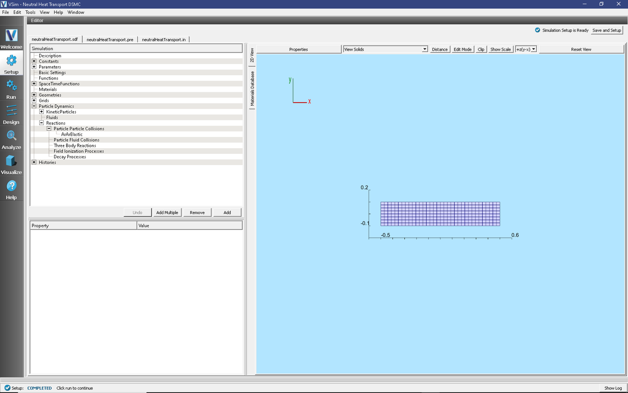
Fig. 570 Setup Window for the Neutral Heat Transport example.
Simulation Properties
This input file contains one kinetic species of neutral Argon, the required thermalizing boundary conditions for the hot and cold plates, and the Ar-Ar elastic collisions. The constants and parameters are set up so that the Argon pressure (ARPRES) in Pa can be changed, and the simulation grid will adjust resolution to ensure that the mean-free path is always resolved. This means that multiple simulations can be run to match the analytic result for a variety of pressures/collisionality.
Running the Simulation
After performing the above actions, continue as follows:
Proceed to the Run Window by pressing the Run button in the left column of buttons.
To run the file, click on the Run button in the upper left corner of the Logs and Output Files pane. You will see the output of the run in this pane. The run has completed when you see the output, “Engine completed successfully.” This is shown in the window below.

Fig. 571 The Run Window at the end of execution.
Visualizing the Results
After run completion, continue as follows:
Proceed to the Visualize Tab by pressing the Visualize button in the left column of buttons.
Select “History” from the Data View drop down menu, which is located in the upper right corner the window.
Two graphs will be shown in the resulting window ( see Fig. 572 ). The first graph, ArEnergy, shows the total kinetic energy of the argon species. The second, AverageEnergyExchange, shows the average energy transferred between the particles and the plates as a function of time. The AverageEnergyExchange plot divided by the cross-sectional area of a plate gives the average heat flux. A python script, validation.py, is provided to calculate this heat flux from the simulation data, and plot the heat flux versus the analytic heat flux. To run this script, go to the examples directory and run python from the command line (using the command “python validation.py”). The first plot is the same histories seen in the VSim Composer visualization. The second plot is the validation.
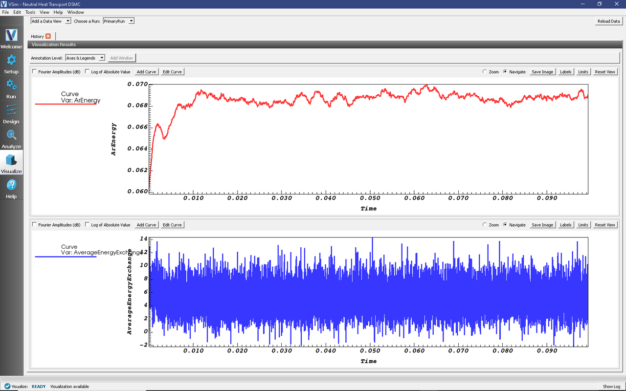
Fig. 572 Results from the history data collected in the simulation.
Further Experiments
As stated in the simulation properties section, simulations can be run with varying pressures (maintaining all else constant) and the resulting heat fluxes plotted against the analytic result, as shown in Fig. 573. The provided python script will only plot one simulation result at a time, but it can be modified easily to overplot multiple simulations. Each simulation should lie on the analytic green line. It is important to ensure that the statistics of the collisions are good enough, so when moving to lower collisionality (pressure) the number of macro particles per cell should be increased. Additionally, it is useful to switch the kinetic particle type so that it is variable weight with managed weights. This allows an isotropic macroparticle density while accounting for a variable physical particle density. Alternatively, the temperature of the plates, distance between them, species of neutral gas, etc. can all be modified to test the generality of the model and collisions.
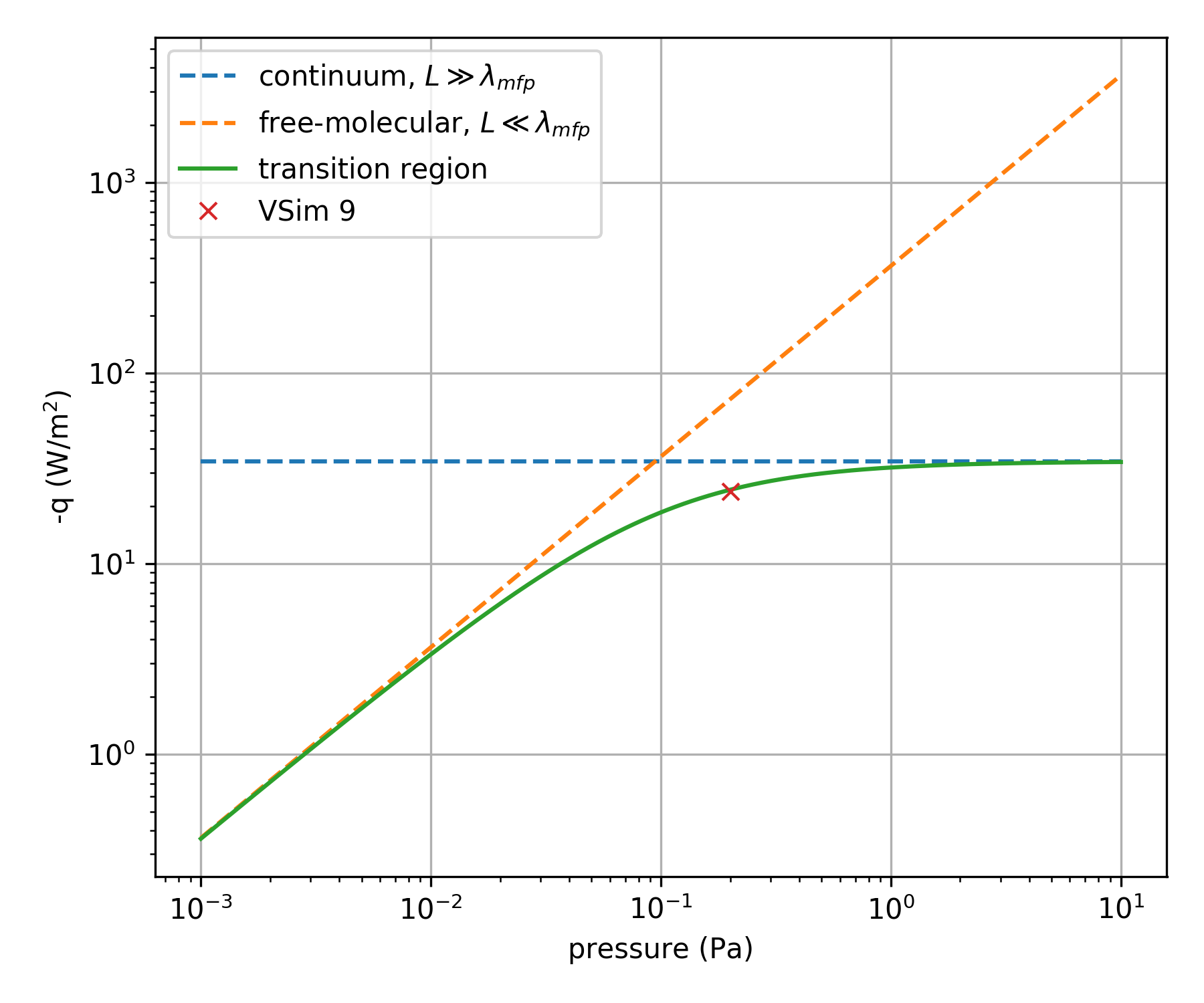
Fig. 573 Analytic result of heat flux compared with simulation.