Corona Discharge 3D (coronaDischarge3D.sdf)
Keywords:
- seed electron population, ionization collisions, poisson solver, dielectric, cascade
Problem Description
This example illustrates how to use VSim to model corona discharge, which is a problem that can occur in a variety of conditions including the manufacturing of dielectrics. In the scenario which we simulate, and which represents many situations, a potential difference is established between two boundaries. In many cases there may also be a dielectric present that can modify the field solution. Furthermore, there will also be an electric field within the dielectric, which VSim correctly calculates. When a potential difference exists between two boundaries, a free electron will be accelerated in the resulting electric field. Free electrons often form due to the ionization of a neutral atom from a stray cosmic ray or UV light. When no potential difference exists, the electron is reabsorbed by surrounding neutrals. However, if a potential difference does exist, this free electron will be accelerated and collide with surrounding neutrals. If the electron ionizes another neutral before being reabsorbed, then a cascade condition is established and more free electrons form due to ionization collisions. This process has been considered by Paschen, who calculated the potential difference required for a cascade of electrons to form. Paschen simplified the process by lumping the contribution from all the collisions into a few terms. However, with VSim, we can consider the effect of each collision separately.
This example illustrates how to set up collisions, and establish a seed electron population (which represents the free electrons that form due to UV light or cosmic rays). We also illustrate a new capability in VSim, which is the ability to create a CSG geometry and assign a dielectric to it.
This simulation can be run with a VSimPD license.
The video attached here provides a full walkthrough of this example: https://www.youtube.com/watch?v=OTBm459OAUo&list=PLottQ0Bg2M-3ATV5O9IP-3TEC4toVYPAK&index=13
Opening the Simulation
The corona discharge example is accessed from within VSimComposer by the following actions:
Select the New → From Example… menu item in the File menu.
In the resulting Examples window expand the VSim for Plasma Discharges option.
Expand the Plasma Processing option.
Select Corona Discharge and press the Choose button.
In the resulting dialog, create a New Folder if desired, then press the Save button to create a copy of this example.
All of the properties and values that create the simulation are now available in the Setup Window as shown
in Fig. 561. You can expand the elements tree and navigate through the various properties,
making any changes you desire. Please note that many options are available by double clicking on an option and
also right clicking on an option. The right pane shows a 3D view of the geometry as well as the grid.
To show or hide the grid, expand the “Grid” element and select or deselect the box next to Grid. You can also
show or hide the different geometries by expanding the “Geometries” element and selecting or deselecting the various
geometries. “cylinderConductorUnionpipe0” is created by performing a boolean union operation between
“cylinderConductor” and “pipe0”.
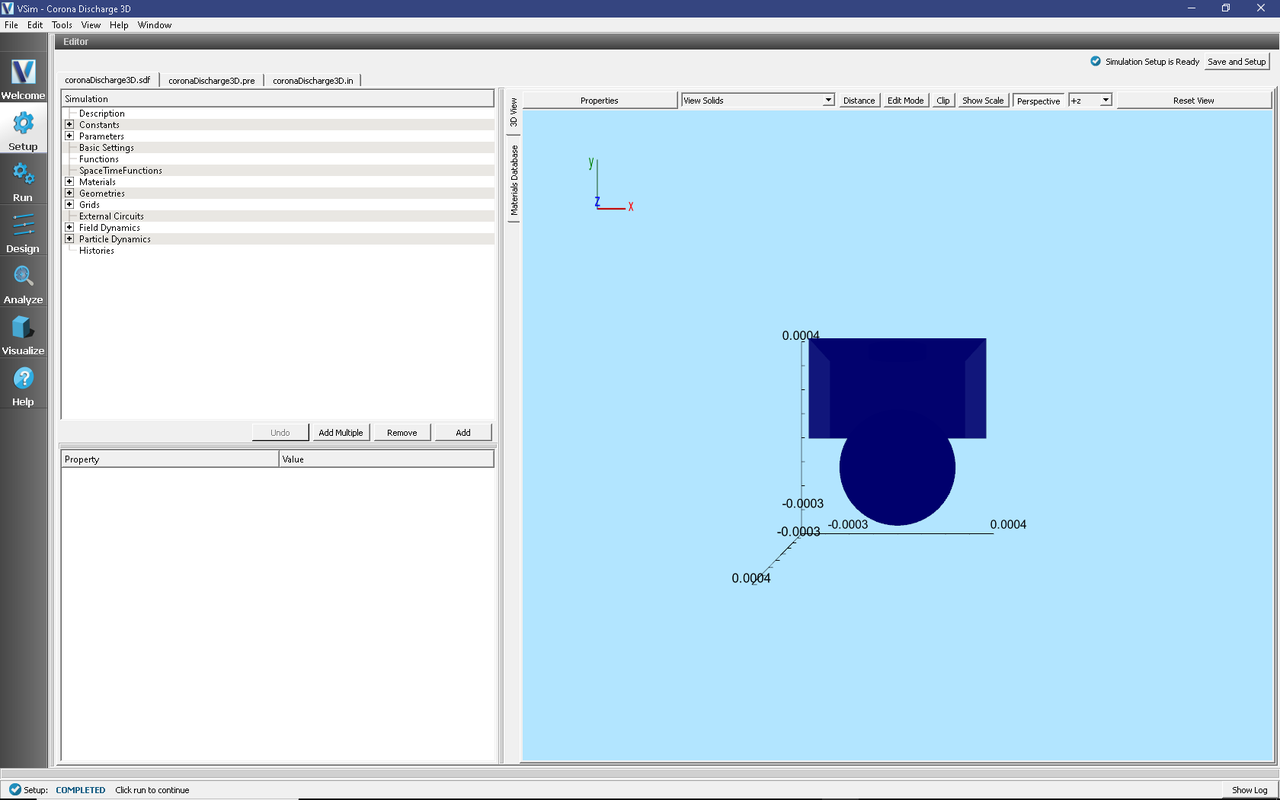
Fig. 561 Setup window for the corona discharge example.
Simulation Properties
This example contains many user defined Constants and Parameters which help simplify the setup and make it easier to modify. The following constants or parameters can be modified by left clicking on Setup on the left-most pane in VSim. Then left click on + sign next to Constants or Parameters and all the constants or parameters used in the simulation will be displayed. To add your own constant or parameter, right click on Constants or Parameters and left click on Add User Defined. Below is an explanation of a few of the constants and parameters used. There are several more constants and parameters included in the simulation.
MAX_SIGMA: Largest cross-section for all collisions that are included in simulation. This sets necessary grid size
GAS_PRESSURE_TORR: Pressure of neutral gas. Mean Free Path (MFP) depends on this
MFP: Smallest Mean Free Path based on GAS_PRESSURE_TORR and MAX_SIGMA. DX/DY/DZ should be less than MFP.
FCOLL: Largest collision frequency. Time step should be smaller than 1/FCOLL
XC_SPHERE/YC_SPHERE/ZC_SPHERE/RADIUS_SPHERE: Coordinates for center of sphere and radius of sphere
CYLINDER_YPOS/CYLINDER_LENGTH/CYLINDER_RADIUS: Coordinates and dimensions for cylindrical dielectric
PIPE_LENGTH/PIPE_OUTER_RADIUS: Dimensions of conductor which surrounds cylindrical dielectric
CYLINDER_CONDUCTOR_YPOS: Y-position of cylindrical conductor that sits on top of the cylindrical dielectric.
Basic Settings
Before creating your own simulation or running an example, a good place to look is the “Basic Settings” in the elements tree. In Basic Settings, you will be able to set the dimensions of the simulation (3D in this case), the type of field solve (electrostatic which is explained more below), whether to include particles and reactions and any periodic directions. You should notice that the x and z directions are periodic in this example.
Importing Materials
All geometries which are included in the simulation must be assigned a material. In VSim 11, a new feature is possible, which is the ability to import a dielectric and assign that dielectric to a geometry. To import a material click on the “Materials Database” button which is below the “3D View” button. I’ve highlighted this window in Fig. 561. To add PEC (for example), click on PEC and the click on “Add to Simulation” at the top of the table. You don’t need to do this since this material is already added, which can be seen by expanding the “Materials” option in the elements tree. We have also added Sapphire, which is the dielectric we have chosen to use. Once these materials are added, they can be assigned to geometries
Geometries Created Using CSG
An important part of this simulation is the creation of several geometries. To view the geometries, left click on the + sign next to Geometries in the Setup window, then left click the + sign next CSG. To view the geometries clearly, you can expand Grid and unclick the box next to Grid. However, there may still be a box present. This is most likely the neutral fluid (which I will explain below). Therefore, expand Particle Dynamics, then expand Fluids and uncheck the box next to “N2”. All the geometries should now be easily viewed. Right clicking anywhere in the “3D View” and moving the mouse allows you to rotate the geometries. A new feature to VSim 11 is the ability to change the scale of the grid which is visualized. At the top of the 3D View, click on “Show Scale”. This will create a scale slider bar at the bottom. Sliding the bar changes the scale that the grid is displayed in. In this simulation, there are two PEC (Perfectly Electrical Conductors) and one dielectric geometry. The two PEC geometries are “sphere0” and “cylinderConductorUnionpipe0”. The latter geometry is created by pressing the “Shift” button and clicking “pipe0” and “cylinderConductor” which highlights the two geometries. Once highlighted, right click and you will see the option to perform a boolean operation. We have already done this to create “cylinderConductorUnionpipe0”. If you click on “cylinderConductorUnionpipe0” or “sphere0”, you will see that the material assigned is PEC. If you click on “cylinderDielectric”, you will see that the material assigned to Sapphire. Assigning a dielectric to a geometry is new to VSim 11 and uses a new electric field solve called cutCellPoisson, which requires a PD license.
Field Boundary Conditions
This simulation solves for the self consistent electric field only (the self consistent magnetic field is not solved for and therefore this field solve is called an “electrostatic field solve”). To solve for the self consistent electric field, the charged particles are interpolated on to a grid, the charge density is computed, and Poisson’s equation is solved at each time step. In order to do this, boundary conditions must be set for all 6 boundaries (since this is a 3D simulation). Since the simulation is periodic along x and y, which we set in Basic Settings, we need to set up boundary conditions at YMIN, YMAX and all PEC geometries. This is done by expanding “Field Dynamics”, then expanding “FieldBoundaryConditions”. Here you will see four Dirichlet boundary conditions, which set the potential along these surfaces. You also have the freedom to set YMIN or YMAX as Neumann (which sets the electric field). Note that either YMIN or YMAX has to have a potential specified in order to invert the Poisson matrix.
Creating Particles
To explore the kinetic species that are included in this simulation, expand “Particle Dynamics”, then expand “KineticParticles”. Here you will see three kinetic species which are “N2Plus”, “seedElectrons”, and “SecElec”. This simulation begins with one seed electron which begins the cascade process that creates the secondary electrons and ionized nitrogen molecules. The seed electrons is called “seedElectrons”. If you expand “seedElectrons”, you will see “particleLoader0”. If you click on “particleLoader0”, you will see that we load one particle on the grid. You can load many more particles if you would like by increasing “macro particles per direction” from (1,1,1) to something larger. Or you can change particle load placement from “grid” to “bit-reversed”, which will load particles randomly in a cell within the region that you establish by expanding “volume”. There are two other kinetic particles that are not initially present. N2Plus and SecElec are both created in the ionization collision seedElectrons + N2 –> N2Plus + SecElec and SecElec + N2 –> N2Plus + SecElec. Both of these collisions can be found by expanding Reactions, then expanding Particle Fluid Collisions and you will see two ionization collisions present. Note that in reality, this simulation should also include elastic collisions and several excitation collisions. We have not included elastic collisions because the mean free path is much smaller than ionization collisions and would therefore require around 20-40 processors to efficiently process. However, in 1D or 2D, including elastic collisions is much more feasible. Finally, we have modeled the N2 is a fluid. You can model a neutral species as either a kinetic particle or fluid.
Running the Simulation
Once finished with the setup, continue as follows:
Proceed to the Run Window by pressing the Run button in the navigation column on the left.
To run the file, click on the Run button in the upper right corner of the Logs and Output Files pane.
You will see the output of the run in that pane. The run has completed successfully when you see the output, “Engine completed successfully.” This is shown in Fig. 562. The simulation takes about 2 hours on 6 cores.
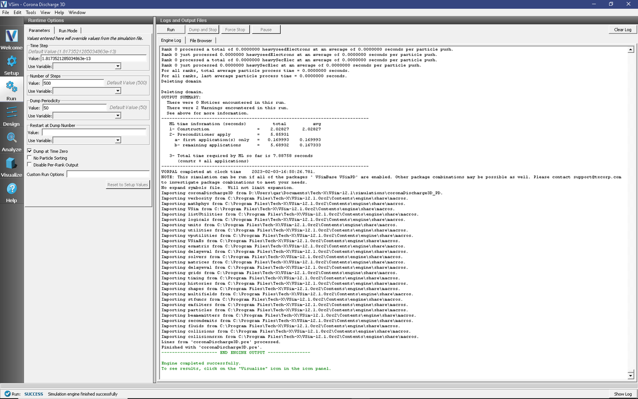
Fig. 562 The Run Window at the end of execution.
Visualizing the Results
After performing the above actions, the results can be visualized as follows:
Proceed to the Visualize Window by pressing the Visualize button in the navigation column.
Clicking on the Add a Data View dropdown menu shows there are many different types of data to visualize.
To get started, lets visualize the self-consistent potential.
Click on the Data Overview tab which is a default tab already loaded in the “Visualize” section of VSim.
Under Variables, expand “Scalar Data” then check the box called “Phi”
To view the potential at a slice through the simulation domain, check the box next to “Clip Plot”
Finally, to visualize the potential superimposed with the geometries in the simulation, expand “Geometries”, and check the boxes next to “poly(cylinderConductorUnionpipe0)”, “poly(cylinderDielectric)” and “poly(sphere0)”.
Slide the bar to the right at the bottom to view the potential as a function of time.
Particles can be superimposed on this plot by expanding “Particle Data” and clicking the species you want to visualize.
The resulting visualization is shown in Fig. 563.
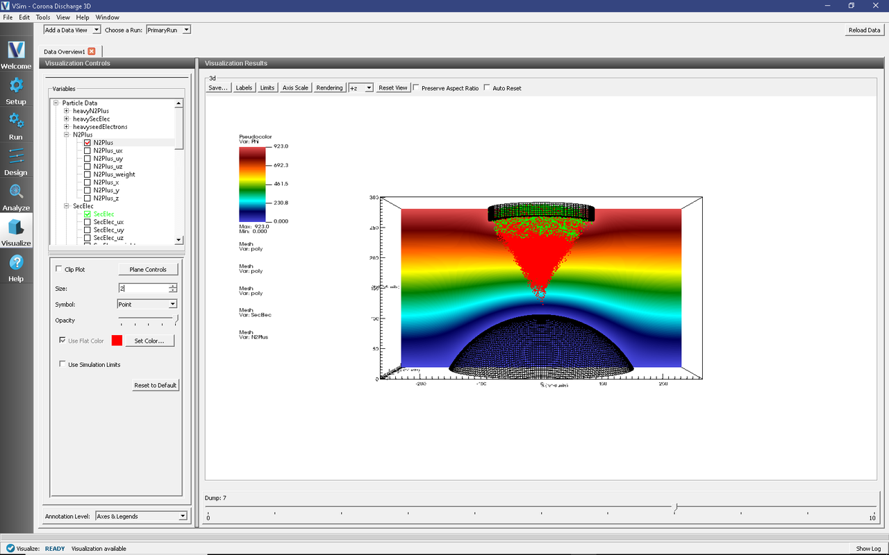
Fig. 563 The evolved potential with the geometries and particles superimposed.
Further Experiments
One way to make the simulation more realistic is to add elastic collisions between N2 and electrons. This will require a smaller cell size to resolve the smaller mean free path. Other collisions that you could add are excitation collisions between N2 and electrons. Examples of excitation collisions can be found in the Townsend Discharge example. If you add more collisions, you will need to add more seed electrons. The reason is that in a given time step, a particle undergoes only one collision (this is an assumption in our model). If you add elastic collisions, the most likely collision to occur will be elastic. Therefore, to increase the likelihood of an ionization collision, you most likely will need to start with several hundred seed electrons. Finally, you can add secondary emission of ions hitting the sphere, which will most likely require several hundred thousand time steps for ions to travel back to the sphere. To include other collisions and a different neutral fluid background, the LXcat scattering database (https://fr.lxcat.net/data/set_type.php) can be used.