Multipacting Resonances in Waveguide (multipactingResonances.sdf)
Keywords:
- multipacting , multipactingResonances
Problem description
Multipacting, which is the resonant buildup of secondary electrons, is often a concern in microwave devices. Anytime there is an oscillating electromagnetic field across a gap between two surfaces there exists the possibility that for the right voltage across the gap a resonance condition will exist allowing the exponential buildup of secondary electrons. A coaxial waveguide is such a structure where these conditions can exist.
This simulation can be performed with the VSimVE license.
Opening the Simulation
The Multipacting Resonances example is accessed from within VSimComposer by the following actions:
Select the New → From Example… menu item in the File menu.
In the resulting Examples window expand the VSim for Microwave Devices option.
Expand the Multipacting option.
Select “Multipacting Resonances in Waveguide” and press the Choose button.
In the resulting dialog, create a New Folder if desired, and press the Save button to create a copy of this example.
The Setup Window is now shown with all the implemented physics and geometries, if applicable. See Fig. 450.
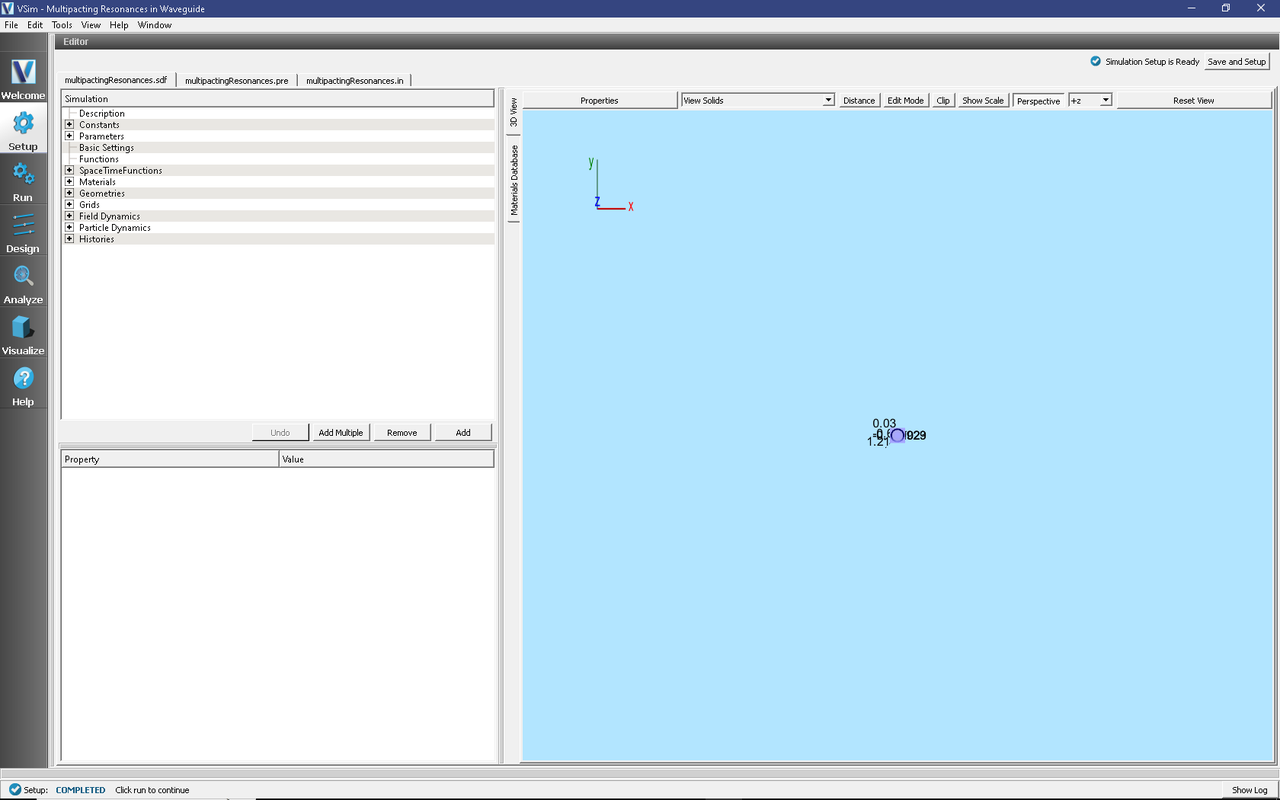
Fig. 450 Setup Window for the Multipacting Resonances example.
Simulation Properties
The input file sets the number of cells along the propagation (x) direction to resolve the wavelength. The electrons are seeded in the middle of the waveguide once the wave has passed. A special electron species is used that allows scans over power to be done in a single simulation. The time step is chosen to be at 90% of the CFL (stability) limit.
Running the simulation
After performing the above actions, continue as follows:
Proceed to the Run Window by pressing the Run button in the left column of buttons.
To run the file, click on the Run button in the upper left corner of the window. You will see the output of the run in the right pane. The run has completed when you see the output, “Engine completed successfully.” This is shown in Fig. 451.
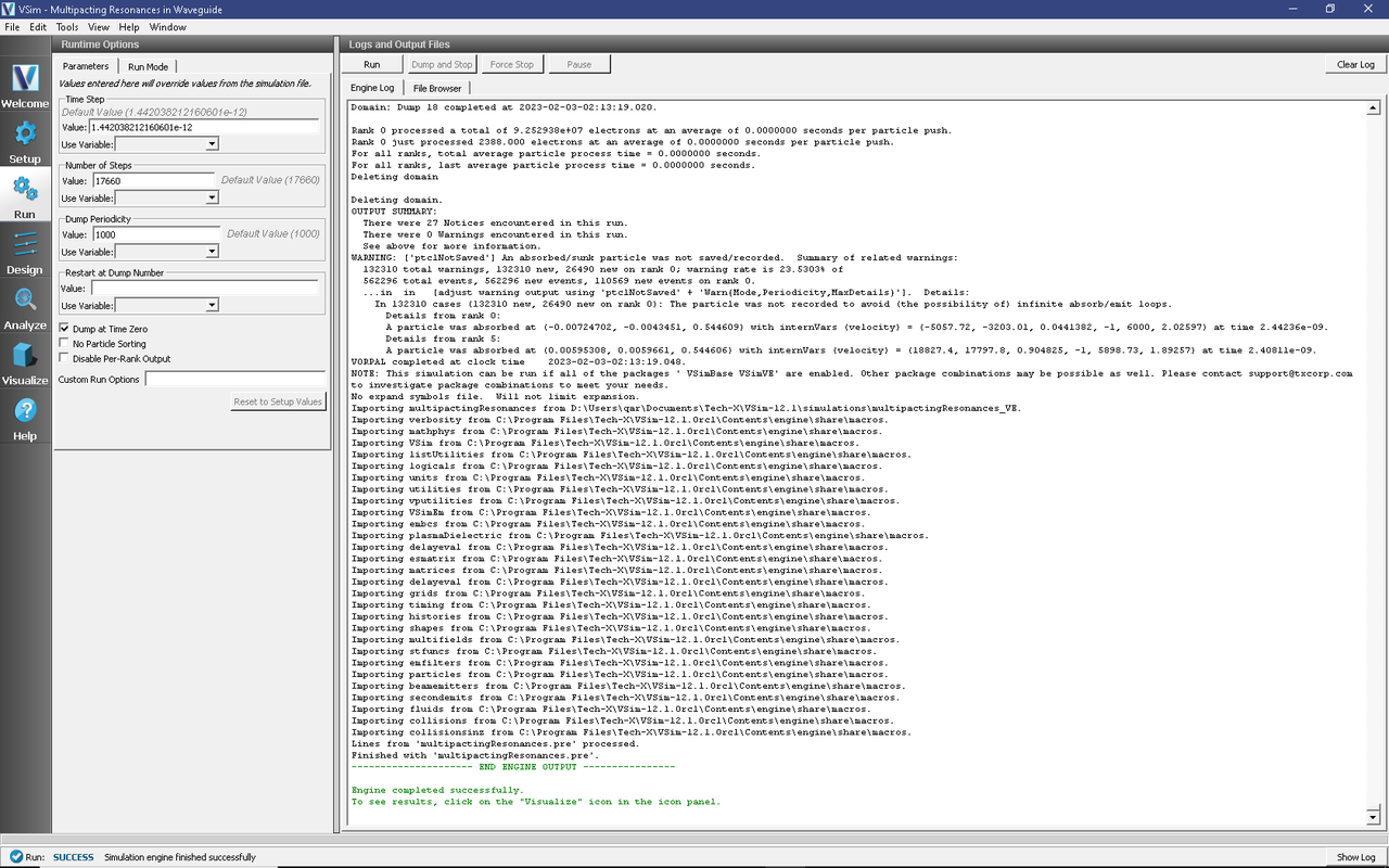
Fig. 451 The Run Window at the end of execution.
Visualizing the results
After performing the above actions, continue as follows:
Proceed to the Visualize Window by pressing the Visualize button in the left column of buttons.
To track the electrons and their field scaled parameters as shown in Fig. 452, proceed as follows:
Select Phase Space from the Add a Data View pull down menu
Select electrons_x for the X-axis
Select electrons_y for the Y-axis.
Select electrons_fieldScaleParam for the Color.
Click on Draw.
Move the Dump slider to Dump: 11.
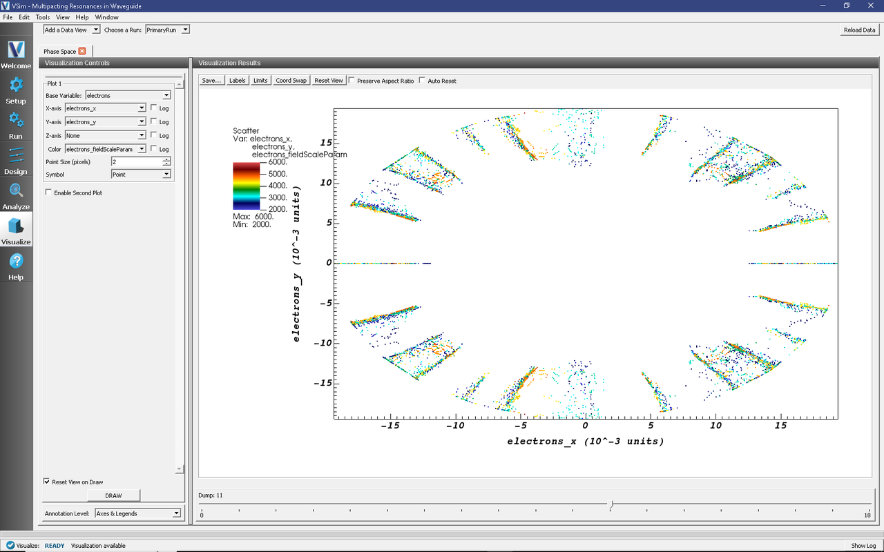
Fig. 452 Location of electrons and their field scaled parameters.
To view growth in the number of electrons, proceed as follows:
Select Binning from the Add a Data View pull down menu
Select electrons_fieldScaleParam for the Dimension 1
Set the bins value to 80, the number of scale factors in the simulation
Select Count for the Operator.
Click on Draw.
Move the Dump slider to the far right.
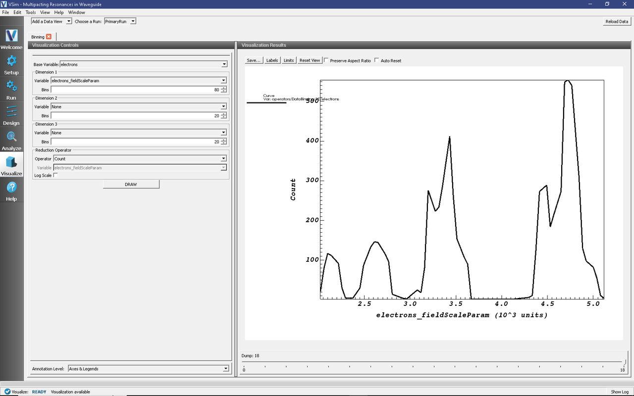
Fig. 453 Visualization of the resonance bands.
Further Experiments
Try seeing how changing the gap voltage or the frequency of the wave changes the multipacting resonances.