Multipacting Growth in Waveguide (multipactingGrowth.sdf)
Keywords:
- multipacting
Problem description
Multipacting, which is the resonant buildup of secondary electrons, is often a concern in microwave devices. Anytime there is an oscillating electromagnetic field across a gap between two surfaces there exists the possibility that for the right voltage across the gap a resonance condition will exist allowing the exponential buildup of secondary electrons. A coaxial waveguide is such a type of structure where these conditions can exist.
This simulation can be performed with the VSimVE or VSimPD license.
Opening the Simulation
The Multipacting Growth example is accessed from within VSimComposer by the following actions:
Select the New → From Example… menu item in the File menu.
In the resulting Examples window expand the VSim for Microwave Devices option.
Expand the Multipacting option.
Select “Multipacting Growth in Waveguide” and press the Choose button.
In the resulting dialog, create a New Folder if desired, and press the Save button to create a copy of this example.
All of the properties and values that create the simulation are now available in the Setup Window as shown in Fig. 447. You can expand the tree elements and navigate through the various properties, making any changes you desire. The right pane shows a 3D view of the geometry, if any, as well as the grid, if actively shown. To show or hide the grid, expand the Grid element and select or deselect the box next to Grid.
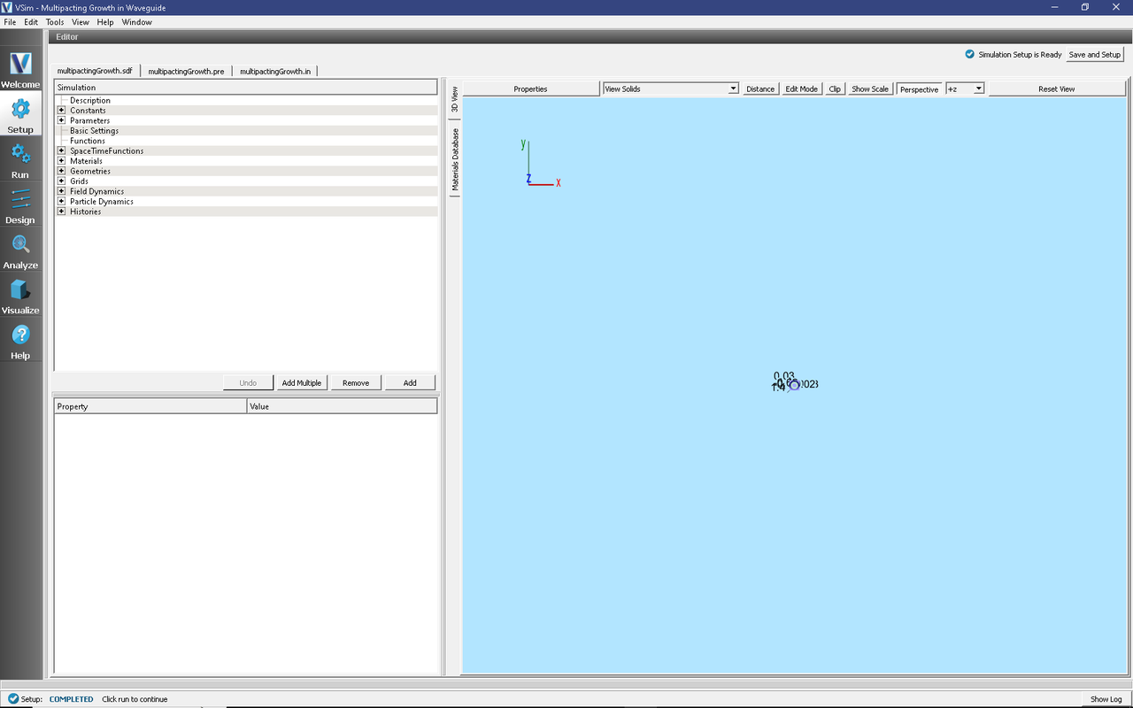
Fig. 447 Setup Window for the Multipacting Growth example.
Simulation Properties
This example contains a number of Parameters to allow for easy manipulation of the device. Those include:
R_O: The outer coax radius
R_I: The inner coax radius
FREQUENCY: The wave launcher frequency
SpaceTimeFunctions are used to create expressions defining the drive frequency and amplitude of the applied field.
CSG is used to create the coax structure by combining cylinders and cubes.
Running the simulation
After performing the above actions, continue as follows:
Proceed to the Run Window by pressing the Run button in the left column of buttons.
To run the file, click on the Run button in the upper left corner of the Logs and Output Files pane. You will see the output of the run in that pane. The run has completed when you see the output, “Engine completed successfully.” This is shown in Fig. 448
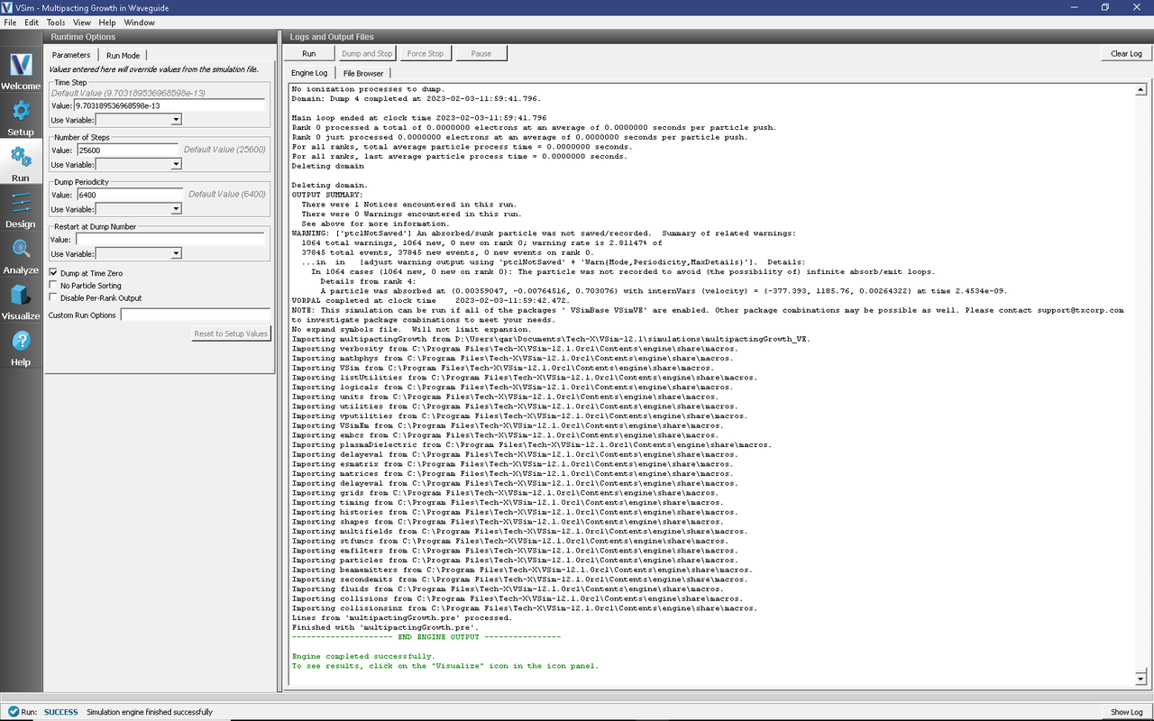
Fig. 448 The Run Window at the end of execution.
Visualizing the results
After performing the above actions, continue as follows:
Proceed to the Visualize Window by pressing the Visualize button in the left column of buttons.
To view growth in the number of electrons, as shown in Fig. 449, do the following:
Select History from the Data View pull down menu
Set Graphs 1&2 to “None”
Graph 3 should already be set to numElectrons (if not, set it)
The overall trend in the number of electrons is an exponential growth with an oscillatory signal that corresponds to the frequency of the traveling wave.
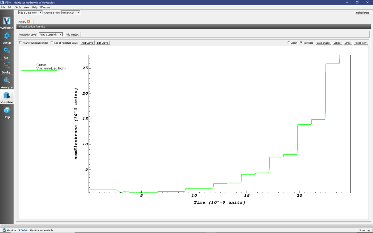
Fig. 449 Visualization of the exponential growth of the electrons due to multipacting.
Further Experiments
Try changing the gap voltage or the frequency of the wave to see if one can take the simulation in and out of resonance.