2D Laminar Brillouin Flow (laminarBrillouinFlowT.pre)
Keywords:
- laminarBrillouinFlowT
Problem description
Many VSimVE applications require a smooth beam to achieve good performance. Simulating such devices can be computationally complex, and commonly we choose to work in 2D instead to save time. In this simulation, we demonstrate how to set up a beam that may be used in the interaction region of any vacuum electronic device you might simulate in 2D, with the interaction structure removed for simplicity.
This simulation can be performed with a VSimVE license.
Opening the Simulation
The Brillouin Flow example is accessed from within VSimComposer by the following actions:
Select the New From Example… menu item in the File menu.
In the resulting Examples window expand the VSim for Microwave Devices option.
Expand the Emission (text-based setup) option.
Select “Laminar Brillouin Flow (text-based setup)” and press the Choose button.
In the resulting dialog, create a New Folder if desired, and press the Save button to create a copy of this example.
The basic variables of this problem should now be alterable via the text boxes in the left pane of the Setup Window, as shown in Fig. 461.
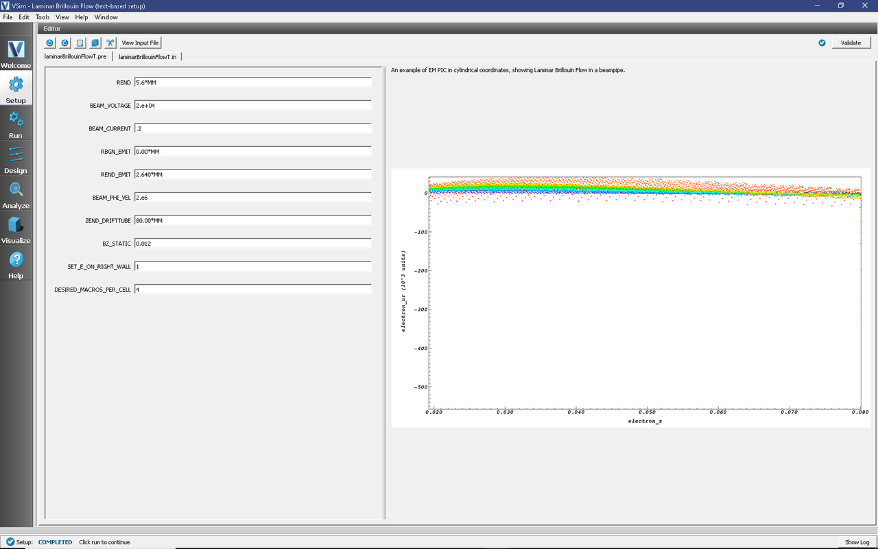
Fig. 461 Setup Window for the Brillouin Flow example.
Input File Features
The Laminar Brillouin Flow example has the following input parameters:
REND is the radial extent of the problem.
BEAM_VOLTAGE specifies the starting voltage for the electron beam.
BEAM_CURRENT specifies the beam current.
RBGN_EMIT and REND_EMIT specify the inner and outer radius respectively of the beam source on the left side of the simulation domain.
BEAM_PHI_VEL sets the rotational velocity of particles at the outside of the beam. Those inside will be given azimuthal velocity proportional to radius.
ZEND_DRIFTUBE determines the amount of beam pipe to simulate.
BZ_STATIC sets the magnetic field (in Tesla)
SET_E_ON_RIGHT_WALL allows for hard-coding a function for the field distribution on the right wall. When set to 1, and the other parameters have default values, the simulation behaves as if the right side of the simulation domain is open. Set to 0, a wall bounds the right side.
DESIRED_MACROS_PER_CELL sets the particle discretization.
Running the simulation
After performing the above actions, continue as follows:
Proceed to the Run Window by pressing the Run button in the left column of buttons.
To run the file, click on the Run button in the upper left corner of the window. You will see the output of the run in the right pane. The run has completed when you see the output, “Engine completed successfully.” This is shown in Fig. 462 below.
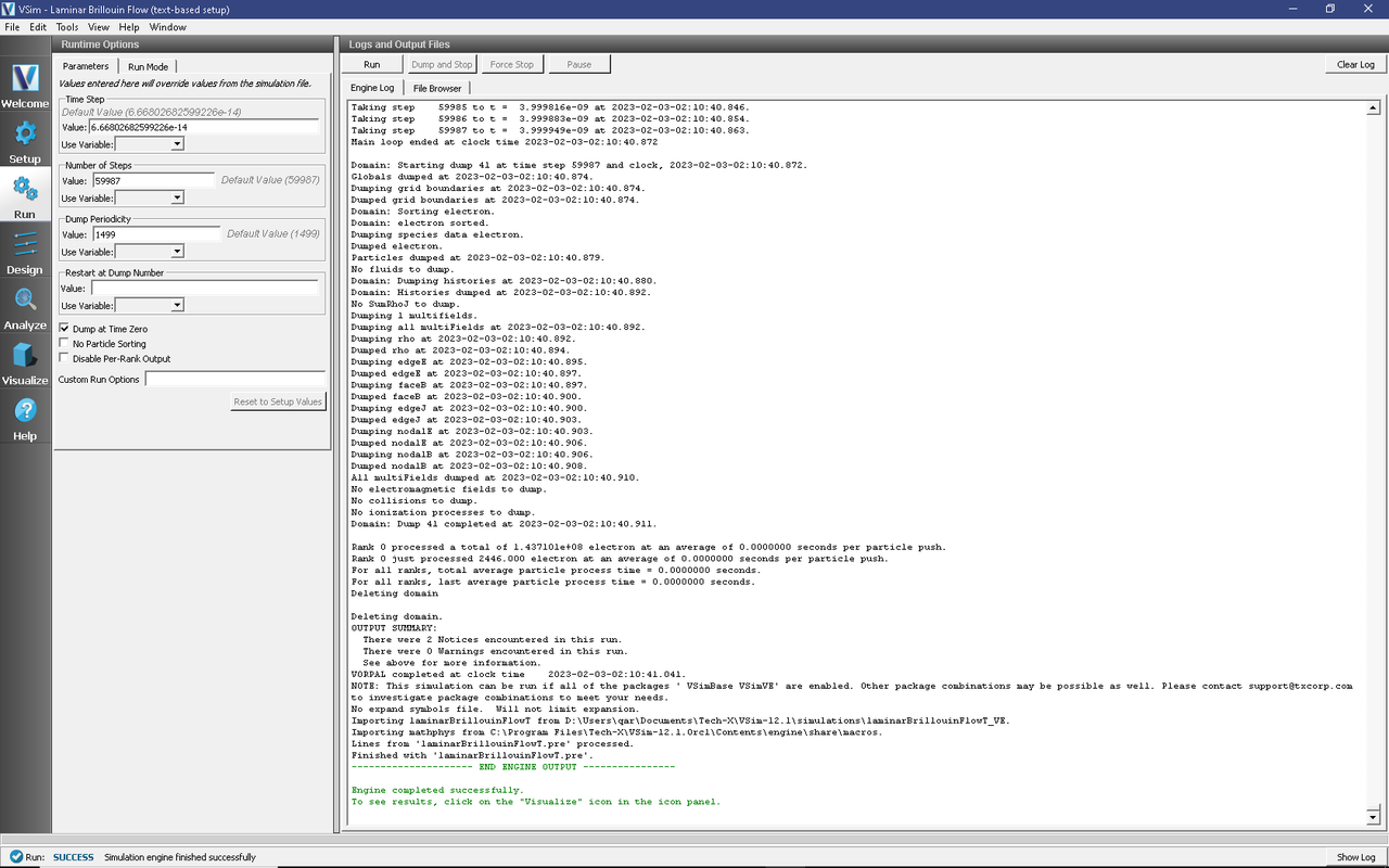
Fig. 462 The Run Window at the end of execution.
Visualizing the results
After performing the above actions, continue as follows:
Proceed to the Visualize Window by pressing the Visualize button in the left column of buttons.
To view the exponential increase in electrons as in Fig. 463:
Select Field Analysis under the Data View drop down
Set the field to edgeE_r
Pull the slider bar to Dump:40
Set the layout to stacked 2d/1d
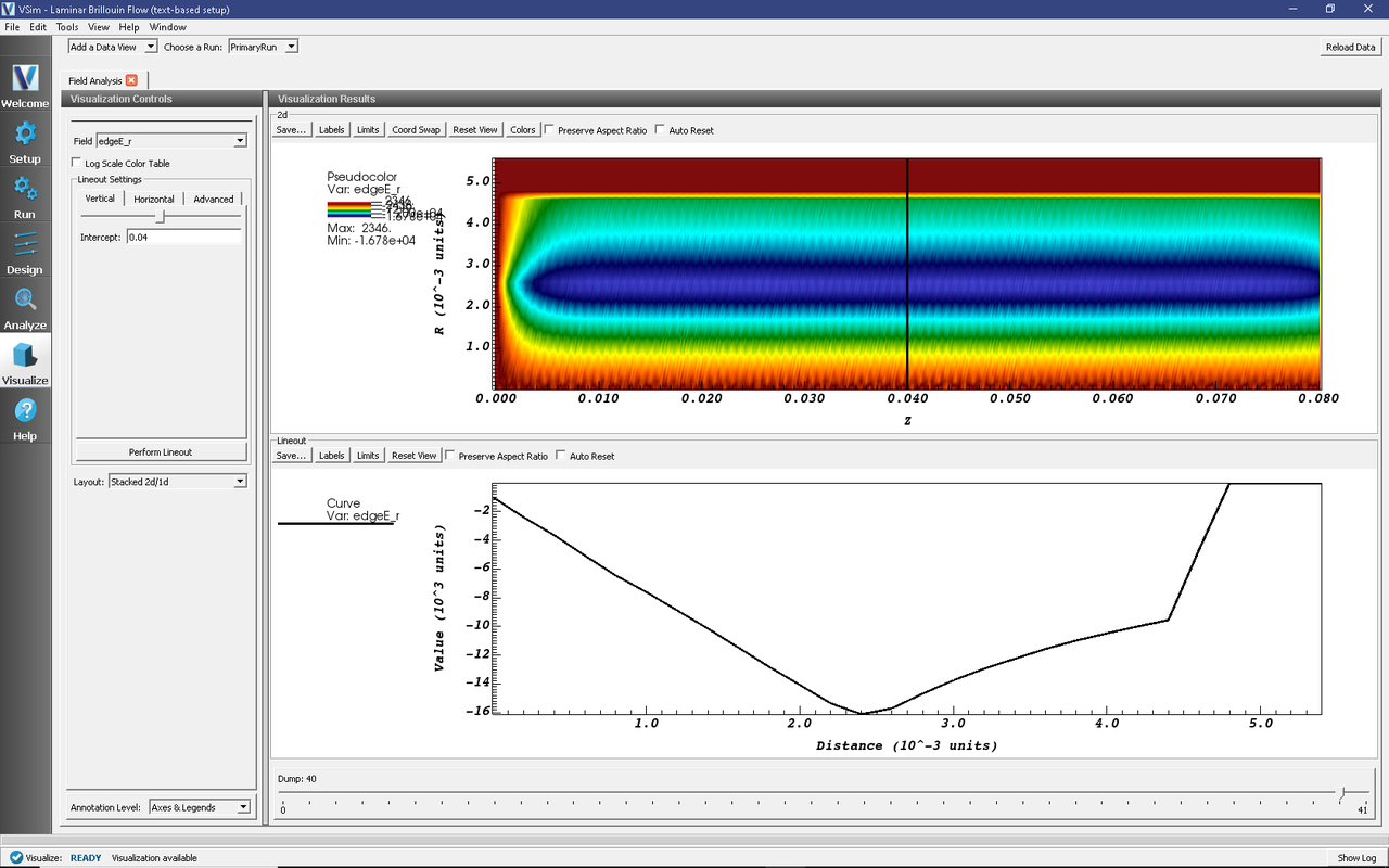
Fig. 463 One can see the transverse field profile.
The transverse field increases with radial distance inside the beam, follows a 1/r distribution outside the beam and rapidly drops to zero at the metal interface.
To view the velocity of the particles in the beam, such as that seen in Fig. 464:
Select Phase Space under the Data View drop down
Set the X-axis to electron_z
Set the Y-axis to electrons_uz
Set the Color to electrons_r
Press Draw.
Move the slide to the right to see how the beam stabilizes.
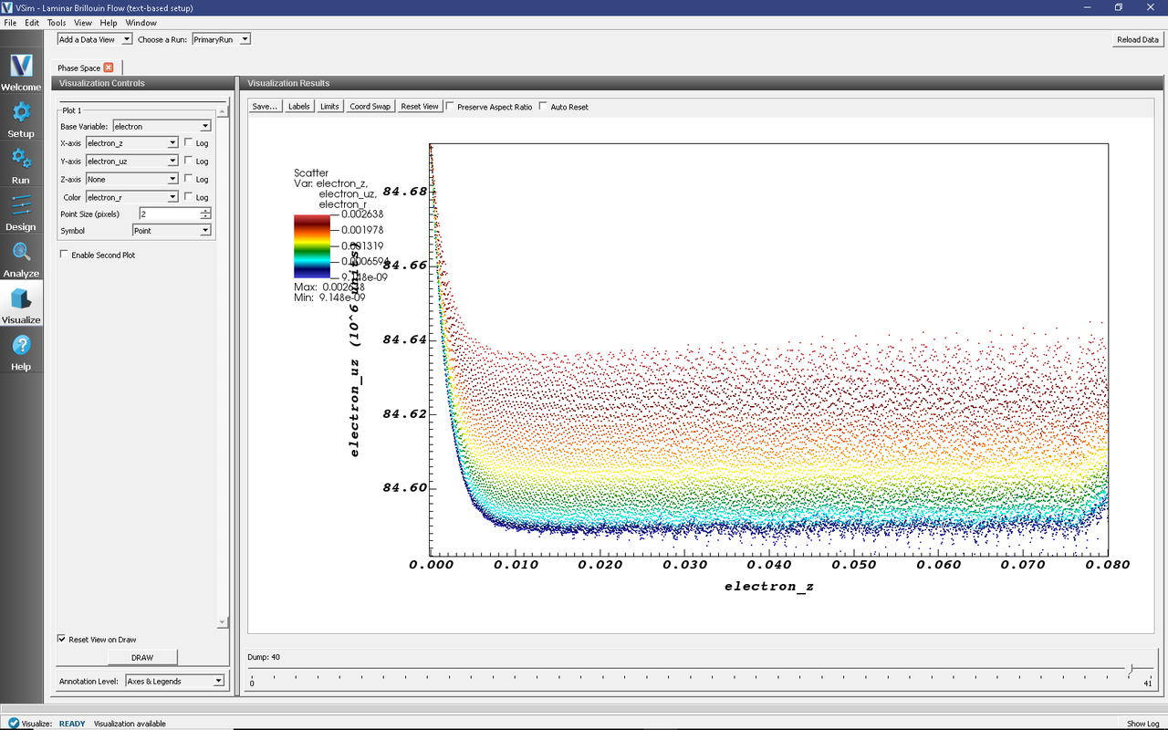
Fig. 464 The beam stabilizes fairly quickly and becomes close to monoenergetic with small transverse velocity.
Switch to beam longitudinal velocity (Y-axis to electrons_uz), and note the orders of magnitude of difference.
Further Experiments
Try varying the starting and ending voltages, and see if the function used to set the right wall needs to be varied, and by how much.