Vaughan Secondary Emission (VaughanSecondaryElecT.pre)

Keywords:

VaughanSecondaryElecT

Problem description

Sometimes secondary emission processes are not adequately explained by the Furman-Pivi model, and sometimes we deliberately wish to compare how simulation results would be affected by different result files. In this example we show how to set up a user defined secondary emission model

Opening the Simulation

The Vaughan Secondary Emission example is accessed from within VSimComposer by the following actions:

• Select the New From Example… menu item in the File menu.

• In the resulting Examples window expand the VSim for Microwave Devices option.

• Expand the Emission (text-based setup) option.

• Select “Vaughan Secondary Emission (text-based setup)” and press the Choose button.

• In the resulting dialog, create a New Folder if desired, and press the Save button to create a copy of this example.

The basic variables of this problem should now be alterable via the text boxes in the left pane of the Setup Window, as shown in Fig. 457.

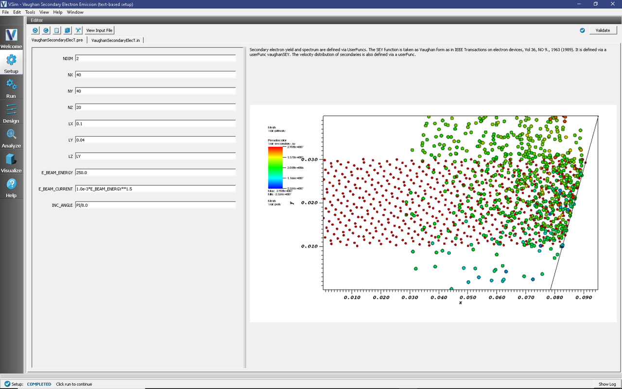
Fig. 457 Setup Window for the Vaughan Secondary Emission example.

Input File Features

The Vaughan Secondary Emission example has the following input parameters:

• NDIM allows adjusting of the number of dimensions

• NX, NY and NZ allow the setting of the number of cells in x, y and z respectively.

• LX, LY and LZ allow the setting of the size of the physical domain to be modeled respectively.

• E_BEAM_ENERGY specifies the energy of the incident electron beam in eV

• E_BEAM_CURRENT specifies the incident beam current

• E_BEAM_ANGLE chooses the angle at which the electrons are incident on a plane surface. We modify the angle of the geometry in this simulation, rather than moving the beam around.

Many of the interesting features in this file require us to click on View Input File.

The userFunc vaughanSEY around line 100 pairs up with

<UserFunc vaughanSEY>
  kind = expression
  inputOrder = [engInc alpha]

in the secondaryEmitter definition. By looking after lines 100 we see how the vaughanSEY arguments are read into this userFunc. We determine the type of data these arguments should contain then build up functions that depend on these arguments. Various terms are built up and then combined in the expression statement

expression= sigmaMax * funcF((engInc - Eth) / (EMax - Eth))

at the end. The second userFunc defines a cosine squared direction distribution, and the third the outgoing energy spectrum.

Running the simulation

After performing the above actions, continue as follows:

• Proceed to the Run Window by pressing the Run button in the left column of buttons.

• To run the file, click on the Run button in the upper left corner of the window. You will see the output of the run in the right pane. The run has completed when you see the output, “Engine completed successfully.” This is shown in Fig. 458 below.

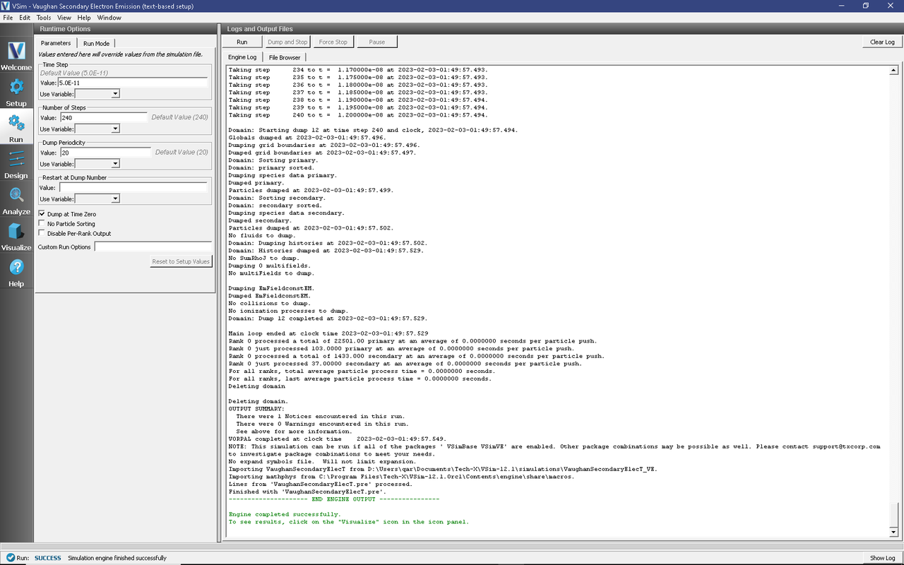
Fig. 458 The Run Window at the end of execution.

Visualizing the results

After performing the above actions, continue as follows:

• Proceed to the Visualize Window by pressing the Visualize button in the left column of buttons.

To view the electrons as in Fig. 459:

• Select Particle Data->primaries and Particle Data->secondaries in the data tree

• If you have a high res monitor you may wish to increase the particle display size in the Size option under Particle Style.

• If you have run the analyzer since visualizing, you will want to click Reload Data before continuing.

• Select Geometries->poly to view the wall with which the particles are colliding.

• Move the dump slider to higher dump numbers to see the particles bouncing off the wall and more secondaries be created.

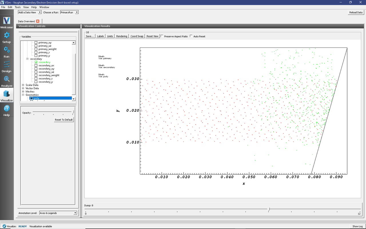
Fig. 459 Visualization of particles hitting the wall in Vaughan Secondary Electron Emission example.

It is also possible to gain information about the effective secondary emission yield, the number of particles out given the particles going in, by comparing the number of primaries and secondaries in the simulation, and the rate at which they are created and lost at steady state.

In this simulation we just start by including histories for the total number of particles of each species, which may be viewed by selecting Histories under Data View in the top left.

Further Experiments

Extra histories have been included to measure the primary electron current absorbed on the wall, and a particle emission history to measure the rate at which the secondaries are coming away. For example with:

<History primCur>
  kind=speciesCurrAbs
  species= [primary]
  ptclAbsorbers = [plateAbsorber]
</History>
<History secCur>
  kind = speciesCurrEmit
  species = [ secondary ]
  ptclSource = secondary.secondaryEmitter
  sourceType = 0
</History>

One can then plot the histories as shown in Fig. 460. To add a history plot, click on Add a Data View, then click on History. You will notice a new visualization tab has been added next to “Data Overview”. To change the font on any of the plots, click on “Tools”, then click on “Settings”, and finally click on “Visualization Options”.

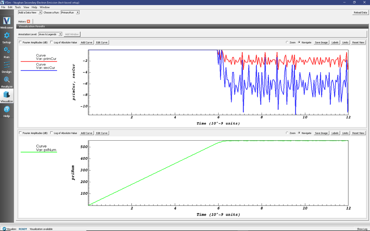
Fig. 460 Visualisation of ratio of primary and secondary particles in Vaughan Secondary Electron Emission example.