Electron Gun (electronGun.sdf)

Keywords:

electron, gun, beam, collimate

Problem description

Electron guns are devices that are often found in vacuum electronics as well as in more advanced technologies such as klystrons, electron microscopes, and particle accelerators. They produce narrow, collimated beams of electrons with precisely tuned kinetic energies. They were often found in cathode ray tubes at the heart of television sets prior to the digital revolution. Electron guns are composed of a cathode, an anode, and repulsive rings. A DC or RF signal is applied to the cathode to produce electrons via thermionic emission. The electrodes produce electric fields that focus the electron beam. Often an additional anode is placed between the cathode and the main anode to act as a repulsive ring that focuses the beam into a small hole in the main anode. The small hole in the main anode acts to collimate the beam.

This example is a specialized electron gun for klystrons and TWTs. It is characterized by high power, a consequence of which is that electrons not successfully collimated can damage the device. To minimize this effect, the gun includes a focusing anode cone, the angle of which is conducive to laminar flow of the electron beam.

Opening the Simulation

The Electron Gun example is accessed from within VSimComposer by the following actions:

• Select the New → From Example… menu item in the File menu.

• In the resulting Examples window expand the VSim for Vacuum Electronics option.

• Expand the Other VE option.

• Select “Electron Gun” and press the Choose button.

• In the resulting dialog, create a New Folder if desired, and press the Save button to create a copy of this example.

The Setup Window is now shown with all the implemented physics and geometries, if applicable. See Fig. 465.

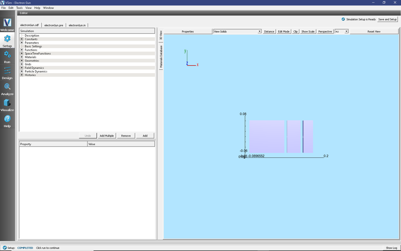
Fig. 465 Setup Window for the Electron Gun example.

Simulation Properties

The input parameters give you total flexibility in defining the geometry of the example. Along with these one can define the nominal cell size, the driving voltages, the strength of the magnetic field, and the beam current.

Running the Simulation

After performing the above actions, continue as follows:

• Proceed to the run window by pressing the Run button in the left column of buttons.

• To run the file, click on the Run button in the upper left corner of the right panel. You will see the output of the run in the right pane. The run has completed when you see the output, “Engine completed successfully.” This is shown in Fig. 466.

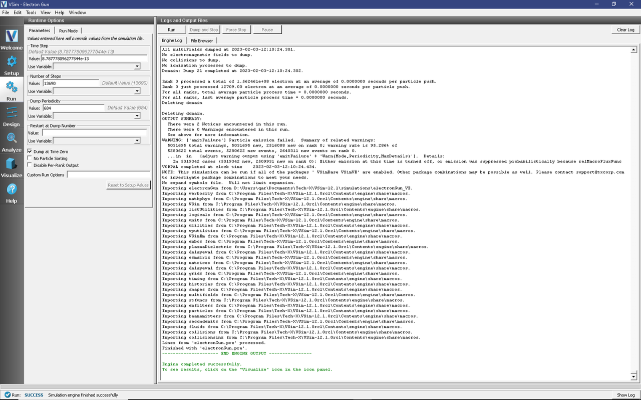
Fig. 466 The Run Window at the end of execution.

Visualizing the Results

To reproduce Fig. 467 proceed as follows:

• Expand Particle Data.

• Expand electron.

• Select electron in red.

• In the lower part of the right pane, move the Dump slider to dump 14.

• Check the “Clip plot” checkbox.

• Expand Scalar Data

• Expand E.

• Select “E_magnitude”.

• In the lower part of the left pane select “Display Contours”.

• Check the “Clip plot” checkbox.

• Expand Geometries.

• Select “poly (electronGunPecShapes)”.

• Check the “Clip plot” checkbox.

This will show the electron beam and the electric and magnetic fields.

The phase space diagram can also be viewed by choosing Phase Space in the Add Data View drop down menu in the top left of the main pane.

The voltages and currents at key locations in the simulation are recorded in Histories and can be viewed by selecting the History data view.

Fig. 467 The electron beam and electric field.

Further Experiments

The geometry is extremely important for proper functionality in this example. For example, the angle that the focusing cone makes with the beam axis determines whether the beam will be laminar. If the beam intersects and diverges, the gun can be damaged by its own power. Try altering the dimensions of the geometry and see the effect on the electron beam.