2D Cartesian Magnetron Sputtering (cartMagnetronSputteringT.pre)

Keywords:

electrostatics, magnetostatics, magnetron sputtering

Problem Description

The 2D Cartesian Sputtering Magnetron simulation models a simple sputtering chamber. For a more extensive reference on magnetron sputtering modeling, see [MI14]. A constant voltage difference is set between two sheets on the upper and lower y boundaries of the simulation domain. The voltage along the left and right walls of the chamber ramp from -500 volts on the bottom boundary (lower y wall) up to 0 volts at the top boundary (upper y wall). To confine the particles, there is a curl-less, divergence-less magnetic field of the form \(\vec{B} = \frac{(y-5*DY)B_{0}}{x^2 + (y-5*DY)^2}\hat{x} - \frac{xB_{0}}{x^2 + (y-5*DY)^2}\hat{y}\). The vertical shift in the y direction moves the singular point of the magnetic field off the origin and below the simulation domain.

The lower x, upper x, and upper y walls are stainless steel, and the lower y wall is copper. A plasma sheath develops above the lower y wall which accelerates argon ions towards the bottom wall. The argon ions strike the lower surface and sputter off neutral copper atoms which ballistically travel through the chamber.

The plasma is sustained through ionization reactions of electrons with a neutral background gas of argon atoms and secondary emission of electrons off all 4 walls of the chamber. The simulation also includes electron-neutral gas elastic and inelastic (excitation) collisions. The Hayashi cross section data from the LXcat database are used with permission from LXcat https://fr.lxcat.net/data/set_type.php.

This simulation can be performed with a VSimPD license.

Opening the Simulation

The cartMagnetronSputteringT example is accessed from within VSimComposer by the following actions:

• Select the New → From Example… menu item from the File menu.

• In the resulting Examples window expand the VSim for Plasma Discharges option.

• Expand the Cartesian Magnetron Sputtering (Text-based setup) option.

• Select cartMagnetronSputteringT and press the Choose button.

• In the resulting dialog, create a New Folder if desired, and press the Save button to create a copy of this example.

The basic variables of this problem should now be alterable via the text boxes in the left pane of the Setup Window, as shown in Fig. 644.

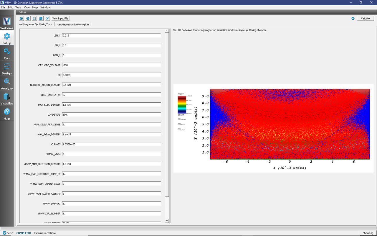
Fig. 644 Setup Window for the cartMagnetronSputteringT example.

Input File Features

This VSimPD example simulates a magnetron sputtering in two dimensions in a Cartesian coordinate. The system size is chosen as 1.5cm x 1.0cm. A nonuniform external magnetic field is applied using the functional field in VSim while the negative voltage is appled through the copper cathode with the rest walls set to ground. Argon is used as the working gas and the plasma dischrage is simulated using the Electrostatic Particle-in-Cell (ESPIC) method with collisions described by Monte Carlo Interactions. The sputtered copper atoms are generated when argon ions hit the copper cathode with enough energy to cause a sputtering.

This simulation can be performed with a VSimPD license.

Running the Simulation

To run the simulation, continue as follows:

• Proceed to the Run Window by pressing the Run button in the left column of buttons.

• Change Number of Time Steps to 20,000 and Dump Periodicity to 200.

• Consider changing ‘Disable Communication Text Files’ (yes, if desired - reduces clutter) in the Advanced tab and ‘Run with MPI’ (yes, if desired - set ‘Number of Cores’ corresponding to your VSim license) in the MPI tab.

• To run the file, click on the Run button in the upper left corner of the window. You will see the output of the run in the right pane. The run has completed when you see the output, “Engine completed successfully.” A snapshot of the simulation run during execution is shown in Fig. 645.

Note

20,000 steps takes about 40 minutes on a MacBook Pro in serial

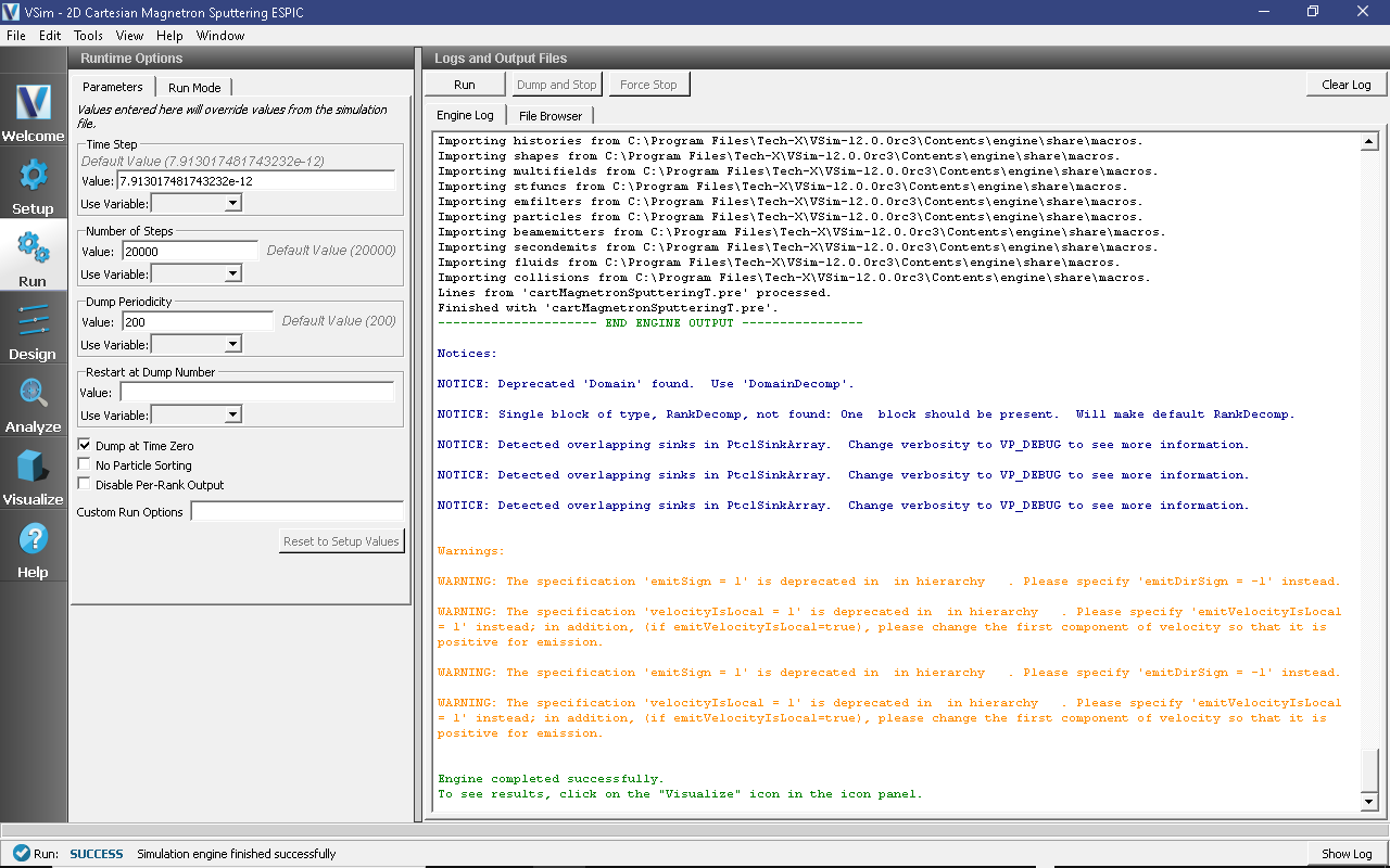
Fig. 645 The Run Window during execution.

Visualizing the Results

Now that we’ve got all of our data, let’s look at it.

• Click the Visualize Window

After a brief moment the visualization options for this data should appear.

We’ll first look at the time evolution of some fundamental one-dimensional quantities. From the Data View pulldown menu on the top left, select History. The default view here should contain four plots, namely, the electron and ion currents to the left wall and the number of electrons and ions in the simulation. A number of notable physics effects can be seen here:

• After a sharp initial decrease in the electron population, the electron population is steady while the ion one declines and the sputtered copper atoms generated. Choose “numMacroArgon”, “numMarcoElec”, and “numMarcoCu” for Graph 1, 2, and 3, respectively. This is not as apparent from the separate numMacroArgon and numMarcoElec plots, but clicking on the “Location” dropdown window in Graph 2 and selecting “Window 1” as the new rendering destination, places both ion and electron populations in the same plot. (Select “<None>” in the plot variable (the topmost menu) for Graph 4 to resize the Argon Ion/electron and Cu plots.) The initial decrease in electron population arises when rapid electron wall losses create a charge imbalance in the plasma and establish plasma sheaths near the walls. Thereafter, this charge imbalance is preserved and the transport of both electrons and ions to the wall becomes ambipolar. A history of the particle populations can be seen in Fig. 646

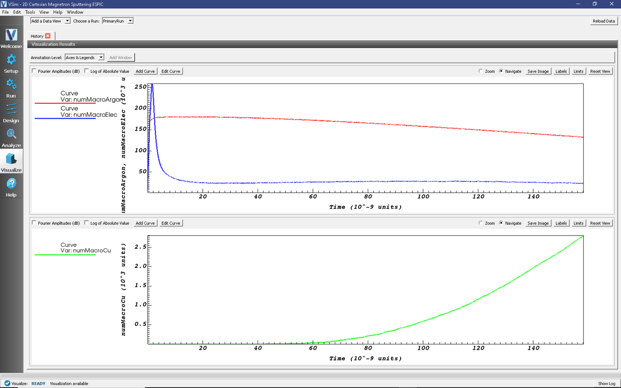
Fig. 646 The electron and ion populations versus time.

We can also look at the plasma and the sputtered copper atoms directly. In the “Data View” menu at the top left of the Composer window, continue as follows:

• Expand Particle Data

• Expand ArgonIons

• Select ArgonIons

• Expand electrons

• Select electrons

• Expand CuNeut

• Select CuNeut

• Expand Scalar Data

• Select Phi

The magnetron sputtering copper atoms can be viewed in the right pane. Use the dump slider on the bottom of the right pane to step through time. After copper atoms are sputtered from the cathode by argon ions, they travel to the anode at their constant inertial velovities as seen in Fig. 647.

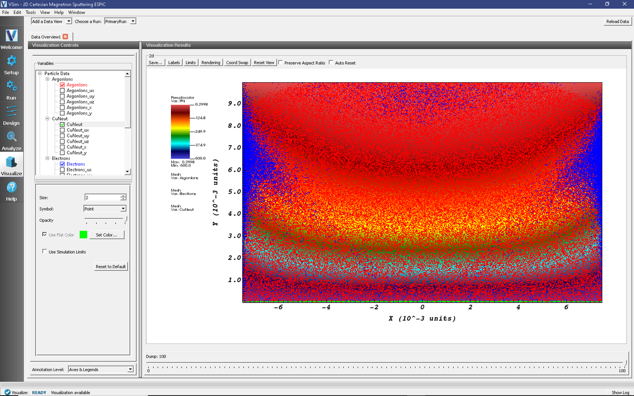
Fig. 647 Plots of this Data View showing the sputtered copper atoms.

The detailed magnetron sputtering can be viewed in the Phase Space. From the Add a Data View pulldown menu, select Phase Space, choose X-axis to CuNeut_x and Y-axis to CuNeut_y and click Draw, as seen in Fig. 648.

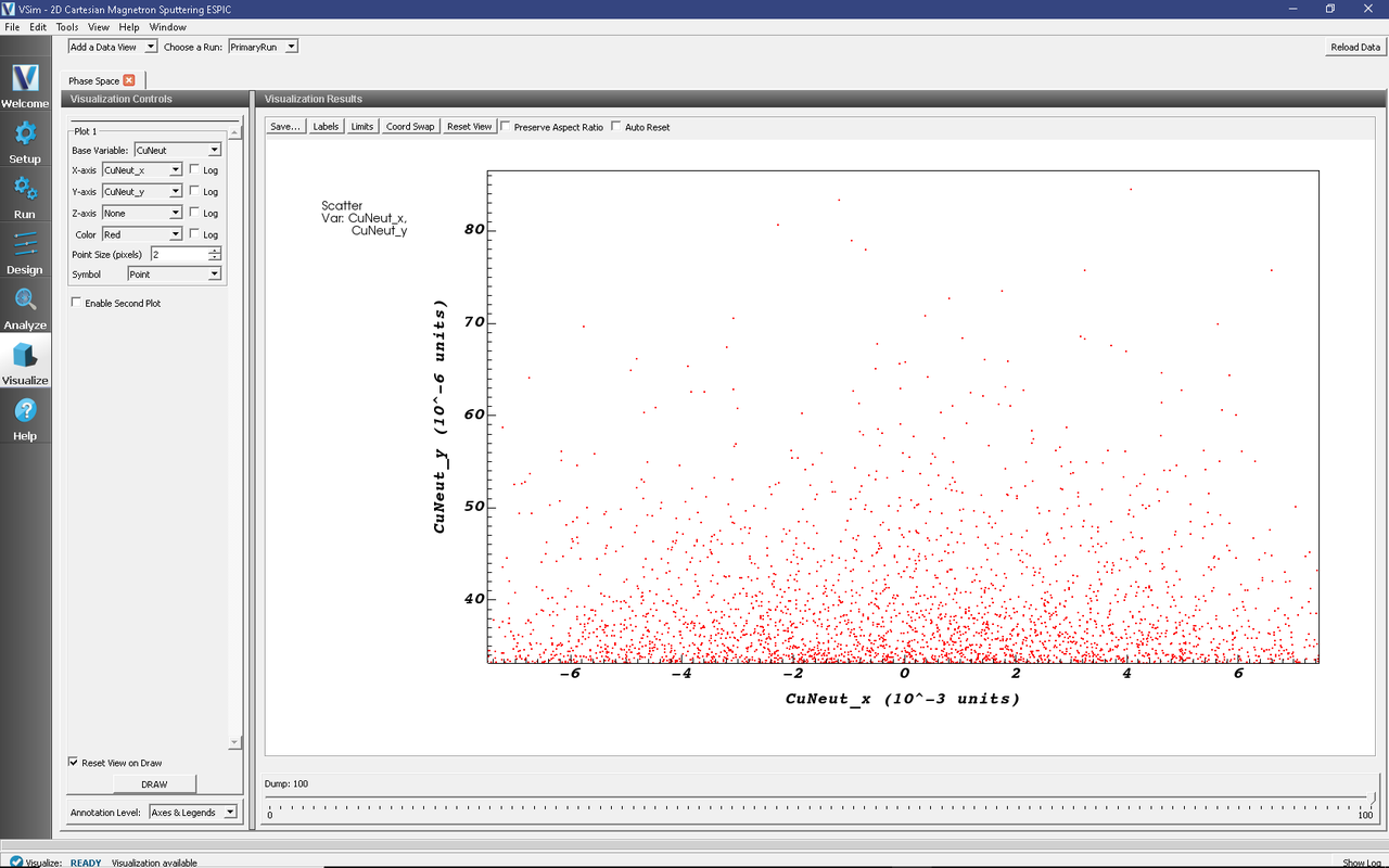
Fig. 648 Plots of this Phase Space showing the sputtered copper atoms travel away from the cathode.

The external magnetic field can be viewed in the Field Analysis. In the Add a Data View menu, select Field Analysis, choose Field to BField_x, as seen in Fig. 649.

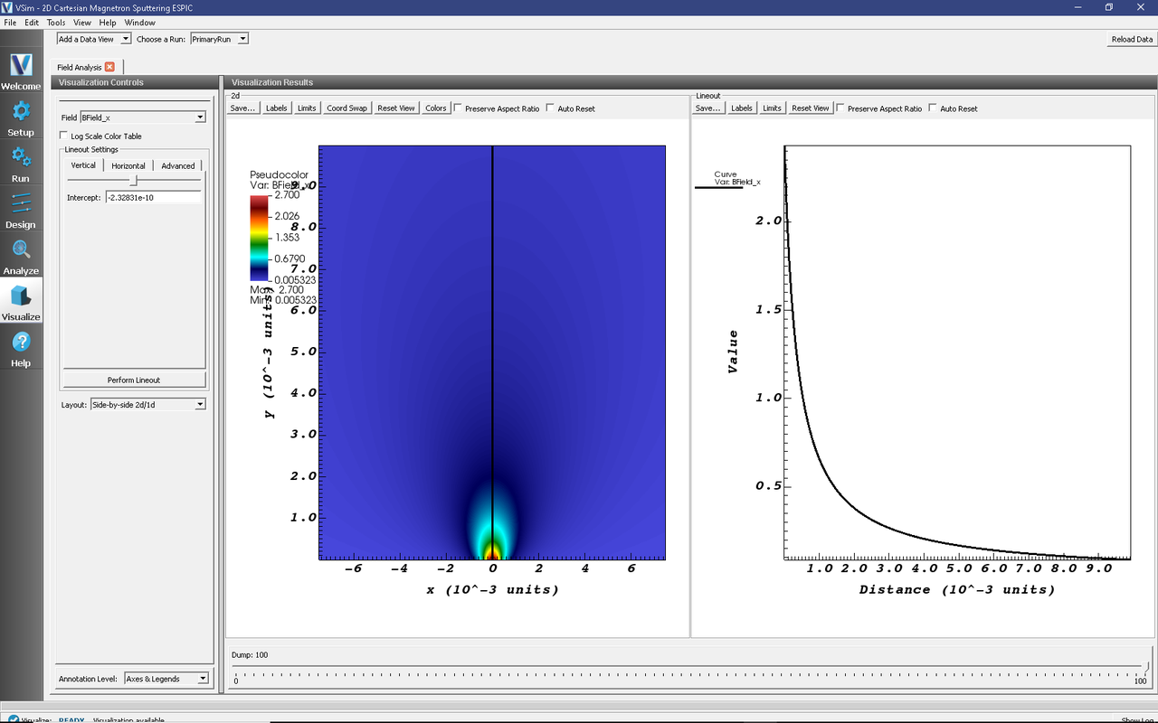
Fig. 649 Plots of this Field Analysis showing the external magnetic field component parallel to the cathode used in the magnetron sputtering.

Further Experiments

1. Add a secondary electron species to track the electrons created through physical processes separately from electrons that were loaded during the initialization period. Be sure to add collisions in the Monte Carlo Block for the new species.

2. Get some new cross-section data from the LXcat

3. Changing magnetic field

Describe something they might see as interesting by changing an xvar value or a value in the Run panel.

References

[1] McInerney, E.J. “Computational Explorations in Magnetron Sputtering.” San Jose, CA: Basic Numeric Press, 2014.