Cylindrical Magnetron Sputtering (cylMagnetronSputtering.sdf)

Keywords:

Poisson solver, secondary electron emission, sputtering, external circuit, external magnetic field, physical vapor deposition, thin film deposition

Problem Description

This example illustrates the use of VSim to model one type of Physical Vapor Deposition (PVD) in which ions are accelerated (via a sheath) onto the cathode leading to the sputtering of the cathode material. The sputtered cathode material (composed of copper) is then dispersed onto the surrounding material uniformly leading to the thin film deposition of copper. There are several key physical concepts which lead to the effective sputtering of copper. The first key concept is that an external magnetic field must supplied in the proper orientation near the cathode. The magnetic field serves to trap some population of electrons which bounce between the north and south poles of two different magnets. The effective trapping of electrons allows for the formation of the sheath. (2) The massive ions are unmagnetized and are accelerated through the sheath onto the cathode. In this process, the ions impart their energy and momentum onto the copper cathode thus releasing copper ions in a process known as sputtering.

In addition, we also seek a steady state solution in this modeling effort. Steady state can be defined in a variety of ways and in this problem, steady state means a near constant number of physical secondary electrons and a near constant cathode potential. The reason for seeking a steady state solution is that PIC models are costly in terms of CPU-hours and many magnetron sputtering industrial setups will run in excess of millisecond time scales. It would take weeks or even months to run on such time scales using a reasonable number of processors. Therefore, if we can find steady state solutions then we can run VSim for 1-10 microsecond on reasonable time scales (less than 24 hours) and on a reasonable number of processors (less than 32) and extrapolate the results to millisecond time scales. Another reason for seeking steady state solutions is physically this will happen in most applications over some time scale. Therefore, by seeking a steady state solution which converges in 1-10 microseconds, we reduce the time it takes to model your problem.

In order to achieve steady state, there are many aspects to this problem which must be balanced. Here we will summarize many of the physical processes which we model and must in turn remain in balance. This problem represents a true multi-physics simulation, all at your disposal in VSim: (1) Collisions between electrons and neutral Ar (2) Secondary emission of electrons off of the cathode (3) Trapping of electrons in the externally supplied magnetic field (4) Floating potential at the cathode modeled using an external circuit (5) Collection of currents at the cathode (6) Sputtering of neutral copper at the cathode

In the following sections, we will explain each part of the setup in more detail and how to modify this example to suit your individual setup.

This simulation can be run with a VSimPD license.

Opening the Simulation

The cylindrical magnetron sputtering example is accessed from within VSimComposer by the following actions:

• Select the New → From Example… menu item in the File menu.

• In the resulting Examples window expand the VSim for Plasma Discharges option.

• Expand the Sputtering option.

• Select Cylindrical Magnetron Sputtering and press the Choose button.

• In the resulting dialog, create a New Folder if desired, then press the Save button to create a copy of this example.

All of the properties and values that create the simulation are now available in the Setup Window as shown in Fig. 635. Note that you can change the scale that is shown on the axes in the Setup window. In this case, the axes in Fig. 635 are shown in cm. You can change the scale by clicking on the “Show Scale” button at the top of the SetUp window. You can expand the tree elements and navigate through the various properties, making any changes you desire. Please note that many options are available by double clicking on an option and also right clicking on an option. The right pane shows a 3D view of the geometry as well as the grid. To show or hide the grid, expand the “Grid” element and select or deselect the box next to Grid.

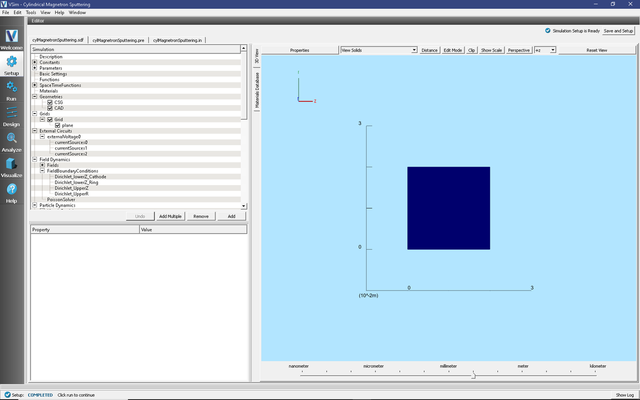
Fig. 635 Setup window for the cylindrical magnetron sputtering example.

Simulation Properties

This example contains many user defined Constants and Parameters which help simplify the setup and make it easier to modify. The following constants or parameters can be modified by left clicking on Setup on the left-most pane in VSim. Then left click on + sign next to Constants or Parameters and all the constants or parameters used in the simulation will be displayed. To add your own constant or parameter, right click on Constants or Parameters and left click on Add User Defined. Below is an explanation of a few of the constants and parameters used. There are several more constants and parameters included in the simulation.

• VOLTAGE0: Initial voltage of Cathode. The Anode is set to 0 V (ground). The Cathode voltage can float by imposing an external circuit model.

• EC_RESISTANCE: Resistance used in external circuit model

• AR_DENSITY: Density of neutral gas (in this case Argon).

• INITIAL_TE_eV/INITIAL_ARPLUS_TEMP: Initial temperature of electron and Ar+ in eV. Simulation results should be somewhat insensitive to this parameter.

There are also several SpaceTimeFunctions (STFunc) defined in this example. MAXWELLIAN_El and MAXWELLIAN_AR are SpaceTimeFunctions used to load the initial Ar+ and electron as Maxwellian velocity distribution functions. In this case the SpaceTimeFunction is actually a function of velocity. Potential_LowerZ_Ring is a function which specifies the voltage in a small region separating the cathode and anode. This function allows for a smooth linear transition in the voltage between the anode and cathode.

You want to run this simulation long enough for the ions, electrons and cathode voltage to come to steady state. As stated in the introduction, we have attempted to reach steady state in 1-10 microseconds. However, your particular setup may take longer. This example ran for about 1.5 microseconds, which is long enough to demonstrate that steady state has been reached. The total number of time steps is 120000.

Explanation of Key Parts of Setup

Setting up the External Magnetic Field Because of the complexity of this problem, we will now further explain key components to this example which are needed to model magnetron sputtering. First, one must include an external magnetic field. There are three ways to include an external magnetic field in VSim. One method (which is the simplest and least general) is to provide an analytic expression as a function of position. You then write this analytic expression as a StFunc. A second method is to use another program to model the magnetic field and write the output into a text file. Then the user can write a space-time Python functions (stPyFunc) to read the data onto VSim and interpolate onto the VSim grid. One example that illustrates this method is the “ionThrusterT” example. A third method is to import a hdf5 file which is vis schema compliant, which is the method we have used in this example. For this example, we used an in-house input file which solves for the magnetic field using a magnetostatic solver via “magnetic charges” and a magnetic scalar potential. The resulting magnetic field can easily be read into VSim by expanding “Field Dynamics” in the setup tree. Under “Field Dynamics”, right click on “Fields”, then choose “Add Field” and finally choose “external field”. This will create a new option under “Fields” with a default name of “externalField0”. By double clicking on “externalField0”, we renamed the external field to “externalMagField”.

Initializing the Plasma If you are creating a simulation from scratch, then you must first enable particles in the simulation. To do this, click on “Basic Settings” in the setup tree. Then find the “particles” option and double click “no particles”, and choose “include particles”. This will create a new option in the Setup Tree called “Particle Dynamics”. By expanding “Particle Dynamics”, then “KineticParticles” in the Setup Tree, the user can see the various kinetic species that are included in this simulation. To create a new species, right click on “KineticSpecies”, choose “Add ParticleSpecies”, and choose either “Charged Particles”, “electrons”, or “Neutral Particles. The species called “electrons” are initially present to initiate the ionization collisions between Argon and electrons which leads to the formation of secondary electrons (secElectrons). The final density of the secElectrons is about 100 times larger than the initial electron density, indicating that the final results in this model are insensitive to the exact initial conditions. The species labeled “ArIons” is used to initialize the simulation in the ionization collision and is also a product in the ionization collisions. Finally, “CuNeut” is the sputtered copper atoms at the cathode. By expanding “electrons”, and clicking on “particleLoader0”, the user can see the necessary parameters for the initial condition. One necessary parameter can be seen by expanding “volume”, which is the spatial location of the initial electron population. It is necessary for the initial electron population to be contained in the boundaries of the simulation domain. You can place the initial population within any volume of the simulation boundaries, and in this case, we choose to fill the entire simulation domain with particles. The user must also specify the initial velocity distribution (i.e. phase space). By expanding “velocity distribution”, the user can see that we have initialized all three velocity components with the same Maxwellian distribution. To population the velocity distribution with a StFunc, simply right on the space next to “u0” and choose the option “assign SpaceTimeFunction” (noting again that this particular SpaceTimeFunction is actually a function of velocity). We also note that a species can be defined without having an initial population such as CuNeut and secElectrons. These two populations form as the simulation progresses in time.

Particle Boundary Conditions When using the visual setup, the default particle boundary condition is set to absorbing in order to prevent particles from leaving the simulation domain (which leads to segmentation faults due to particles entering a region of memory not controlled by VSim). The exception to this default boundary condition is the lower R boundary condition in an axi-symmetric simulation, which defaults to specular (and does not need to be set up in the visual setup). User supplied boundary conditions can be set up by right-clicking on a species (such as “electrons” or “secElectrons”), clicking on “Add ParticleBoundaryConditions”, and choosing one of the many options available. Each specific boundary condition is discussed in greater detail in the Reference Manual. In this model, we have used either “Boundary Absorb and Save” or “Interior Absorb and Save”. Cut-Cell boundary conditions can be used on geometries. To set up a particle history, the user must first set up an “Absorb and Save” particle boundary condition. We note one particular particle boundary condition called electronsabsSaveCathode, secElectronsabsSaveCathode, and ArIonsabsSaveCathode. These three boundary conditions are needed to set up the external circuit, which is discussed below. To see where these three particle boundary conditions are used, we now navigate to “Histories”.

Setting up Histories A “history” is data collected at every time step. There are several histories set up in this example. By expanding the “Histories” option, the user can see all the histories that are set up in this example. To understand how to set up this history, right click on “Histories” revealing all the different types of histories available in the visual setup. If the user hovers the mouse over “Add ParticleHistory” and clicks on “Absorbed Particle current”, a new history will be created. Double clicking on the new history allows the user to change the name of the history. Now left-click on the newly created history and the user will see an option called “particle absorber”. Left clicking “please select” reveals all the particle boundaries that have been assigned “Absorb and Save”. Therefore, to use the “Absorbed Particle Current” history, the user first has to setup at the “Absorb and Save” particle boundary condition. Three useful histories are called “ionCathCurr”, “elecCathCurr”, and “secElecCathCurr”, which are the currents for the three plasma populations that are collected on the cathode at every time step.

Setting up the External Circuit To specify the field boundary conditions discussed in the next paragraph, we must first discuss the external circuit model. This model can be conceptually understood as an external circuit which connects the cathode and the anode. In the circuit model, we include a resistor, with the value of the resistor specified by the user. Obviously the resistance needs to be greater than 0 to make physical sense. The relation between the cathode voltage and the current is simply given by Ohm’s law. Therefore, to fully specify the current, we must compute the current accumulated on the cathode at each time step, which was discussed in the previous paragraph. The external circuit model can be set up by right clicking on “External Circuits”, and choosing the option “Add Resistive Voltage Source”. This will create a new option called “externalVoltageN”, where “N” is some integer. Next right click on “externalVoltageN” and click on “Add Boundary Condition”. This will create a new option under “externalVoltageN” called “currentSourcesN”. Now click on “currentSourcesN”, and choose the boundary condition that contributes to the current on whatever boundary you choose (in our case the cathode). Repeat this process for all the plasma particles that contribute to the current. In our circuit model, we have included the contribution of electron, secElectron, and ArIons currents. Finally, to finish the external circuit model, the user needs to specify the resistance (in Ohms), and a parameter called “Time Constant”. This last parameter is used to create a low pass filter. Since particle codes are noisy, we want to average the current over some number of time steps and use this average value to specify the current. “Time Constant” specifies the number of time steps to average over.

Setting up Field Boundary Conditions Next we discuss the field boundary conditions, which are found by expanding “Field Dynamics” then expanding “FieldBoundaryConditions”. This simulation is electrostatic which means that we only solve the self-consistent electric field and assume that the self-consistent magnetic field does not contribute to the plasma dynamics. Therefore all boundaries (except lower R) need to be assigned either the value of the potential (Dirichlet) or the electric field (Neumann). In an axisymmetric simulation (such as this example), lower R is a computational construct and therefore (in almost all simulations) does not represent a real physical boundary. Therefore, lower R is not assigned by the user and is given a default Neumann boundary condition. Right clicking on “FieldBoundaryConditions” exposes either the “Neumann” or “Dirichlet” options. To see where the external circuit model is used, click on “Dirichlet_LowerZ_Cathode”, where the user can see “externalVoltage0” populates the “boundary surface” option. Therefore, this potential will float based on the total current at the cathode. To summarize the steps needed to include an external circuit in an electrostatic simulation:

1. Set up particles with “Absorb and Save” boundary condition.

2. Right click on “External Circuit” to add a new external circuit.

3. Right click on the newly created option to add a particle boundary condition. Make sure to do this for every particle impacting a surface.

4. Populate “resistance” and “time constant”.

5. This external circuit can now be used as a Dirichlet boundary condition under “Field Dynamics”.

NB: Following these steps creates new histories which can be visualized during or after the simulation has run.

Setting up Reactions If you are creating a simulation from scratch, then you must first enable reactions in the simulation. To do this, click on “Basic Settings” in the Setup Tree. Then find the “collisions framework” option and double click “no collisions”, and choose “reactions”. Note that you must first add particles in order to add collisions. This will create a new option under “Particle Dynamics” called “Reactions”. Since we are modeling the Argon as a neutral fluid (as opposed to a neutral particle), then you will notice all the collisions are “Particle Fluid Collisions”. The user can add new collisions by right clicking on “Particle Fluid Collisions” and choosing one of the many collisions. All collisions require a user supplied cross-section table. For this example, we have supplied the cross-section tables for the reactions. The cross-section tables in the reactions framework contain two columns. The first column is electron energy in eV. The second column is the cross section in \(\textrm{m}^2\).

Setting up Secondary Emission off Cathode The particle population called secElectron is produced from ionization collisions between electrons and neutral Argon and also from secondary emission off the cathode. In this model, we include secondary emission from both electrons and Argon ions impacting the cathode. The secondary electron emission model is based on [FP02b]. To setup secondary electron emission, first create the species using the method discussed in the section called Initializing the Plasma. Then right click on the newly created species, hover your mouse over “Add ElectronEmitter”, then click on “Secondary Emitter”. Following these steps will create a new option called “secondaryElectronEmitter0” which can be renamed by double clicking on the newly created option. Under the secondary electron emitter option, double click next to “emitter boundary type” and choose which type of boundary you want to emit from. If you choose “boundary emitter”, then “material properties” next to “emission specification”, the user can choose either copper or stainless. Finally, the user needs to select which boundary to emit from which is done under “particle boundary condition”.

Setting up Sputtered Copper The particle population called “CuNeut” is created from copper sputtering off of the copper cathode. This population can be setup by first creating a kinetic neutral species. Once the neutral species is created, right click on the species name, select “Add NeutralEmitter” and select “Sputter Emitter”. A new emitter will be created called “sputterNeutralEmitter0”. Click on the newly created sputter emitter and the region next to “particle boundary condition” to select the boundary that you want to emit from. Since this is a sputter emitter, make sure the particle boundary condition corresponds to an ion hitting the boundary.

Running the Simulation

Once finished with the setup, continue as follows:

• Proceed to the Run Window by pressing the Run button in the navigation column on the left.

• To run the file, click on the Run button in the upper left corner of the Logs and Output Files pane.

You will see the output of the run in that pane. The run has completed successfully when you see the output, “Engine completed successfully.” This is shown in Fig. 636.

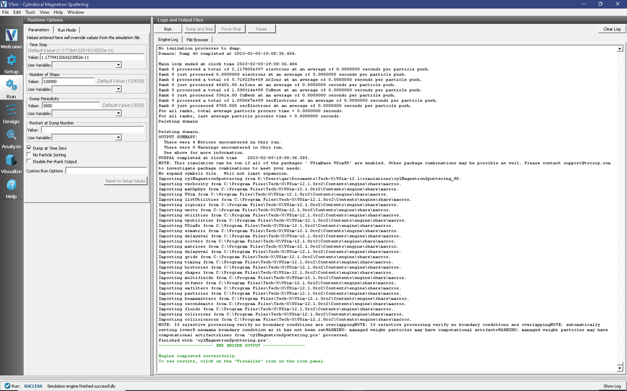
Fig. 636 The Run Window at the end of execution.

Analyzing the Results

Every VSim software purchase comes with numerous post-processing routines written in Python which we call analyzers. For this example, we demonstrate the use of 3 analyzers which computes the electron temperature and density, and the copper density. The name and use of each analyzer is discussed below.

Step 1A: After the simulation has completed, continue as follows:

• Proceed to the Analysis Window by pressing the Analyze button in the navigation column.

• There should be three pre-selected, pre-populated analyzers already loaded. However, if the this is not the case, follow these steps:

• In the resulting list of Available Analyzers, select addSpeciesWithKinEnrgInEV.py and press Open

• The analyzer fields should be filled as below:

  • simulationName: cylSputteringMagnetron

  • species: secElectrons

  • outputSpeciesName: WithKinEnrg

Select the boxes “Remove”, “outputMagnitude”, and “overwrite”. De-select the boxes “outputXcomponent”, “outputYcomponent”, and “outputZcomponent”. This analyzer creates a new data set called “secElectronsWithKinEnrg” and has a “.vsh5” extension to indicate that this data set is computed with an analyzer (all data sets generated from analyzers have .vsh5 extensions. These files are saved in the hdf5 standard).

• Click Analyze in the top right corner.

• The analysis is completed when you see the output shown in Fig. 637.

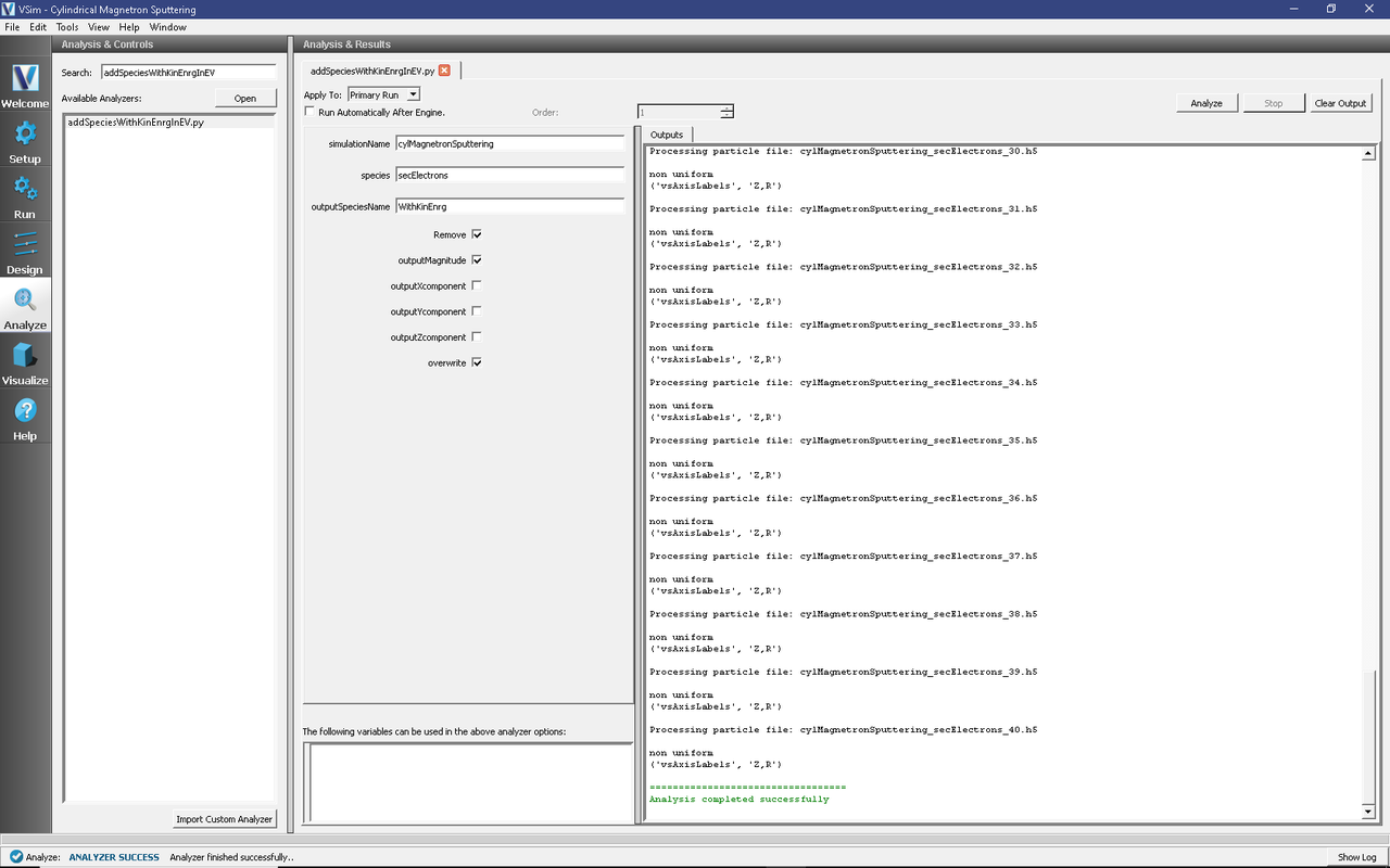
Fig. 637 The Analyze Window showing the use of addSpeciesWithKinEnrgInEv.py.

The resulting data set contains the total kinetic energy of each particle appended on the original particle data. If the particle has a small drift, then the total kinetic energy can be used to compute the temperature. addSpeciesWithKinEnrgInEV.py needs to be run before the next analyzer can be run.

Step 1B: After running the addSpeciesWithKinEnrgInEV.py in Step 1A, continue as follows (Note: if computeDebyeLength.py is already open and populated simply click “Analyzer” in the upper right corner).

• In the resulting list of Available Analyzers, select computeDebyeLength.py and press Open

• The analyzer fields should be filled as below:

  • simulationName: cylSputteringMagnetron

  • species: secElectronsWithKinEnrg

• Click Analyze in the top right corner.

• The analysis is completed when you see the output shown in Fig. 638.

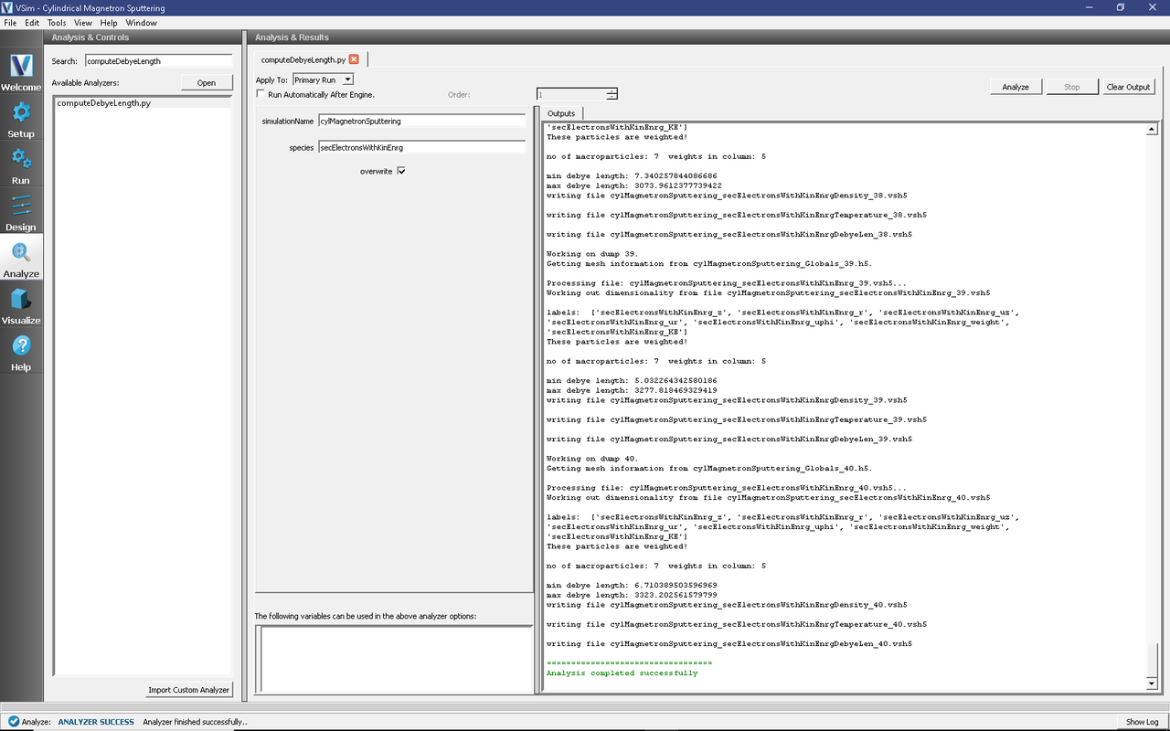
Fig. 638 The Analyze Window showing the correct use of computeDebyeLength.py.

This analyzer produces three new data sets. The data set called secElectronsWithKinEnrgDensity contains the secondary electron density in MKS units. The data set called secElectronsWithKinEnrgTemperature contains the secondary electron temperature in Kelvin. Finally, the data set called secElectronsWithKinEnrgDebyeLen contains the ratio of the secondary electron Debye length to the smallest cell size which must be greater than 1 everywhere in order to obtain physically meaningful results. As already stated, Step 1B requires you to first run Step 1A. The next step (Step 2) can be run independently.

Step 2: If the analyzer computePtclNumDensity.py is not already open, follow these steps.

• In the resulting list of Available Analyzers, select computePtclNumDensity.py and press Open

• The analyzer fields should be filled as below:

  • simulationName: cylSputteringMagnetron

  • species: CuNeut

  • avgNxN: 1

  • iterateAvg: 1

  • timeAvg: 1

  • species: CuNeut

  • minDumpNum: N/A

  • maxDumpNum: N/A

• Click Analyze in the top right corner.

• The analysis is completed when you see the output shown in Fig. 639.

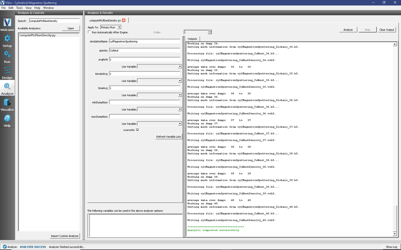
Fig. 639 The Analyze Window at the end of computePtclNumDensity.py.

This analyzer computes the copper density in MKS units. It contains several useful features such as the ability spatially and temporally average the data.

Visualizing the Results

After performing the above actions, the results can be visualized as follows:

• Proceed to the Visualize Window by pressing the Visualize button in the navigation column.

• Clicking on the Add a Data View dropdown menu shows there are many different types of data to visualize.

• To get started, lets visualize two history plots which demonstrate that the simulation has reached steady state.

• If a History tab is not already open, then left-click on History

• Two windows should be open on the pre-loaded History tab which shows cathode voltage on the top plot and number of physical electrons on the bottom plot. If the History tab is not pre-loaded, then follow these next steps:

• After opening a new history tab, there should be two windows present.

• On the top plot, left-click on “Add Curve” and add the data set called “externalVoltage0RealVoltage”. This is the cathode voltage

• Then click on “Edit Curve”, and click on “Select Curve” in the window that pops up. If a second data set is plotted, delete that data set.

• For the bottom plot, follow similar steps: Click on “Add Curve” and add the data set called “numPhysElec”. This is the number of physical electrons modeled in the simulation.

• If a second data set is present, click on “Edit Curve” and delete the second data set.

• We used the “Labels” option on the upper right corner to label the y-axis on the cathode voltage history plot

The resulting visualization is shown in Fig. 640.

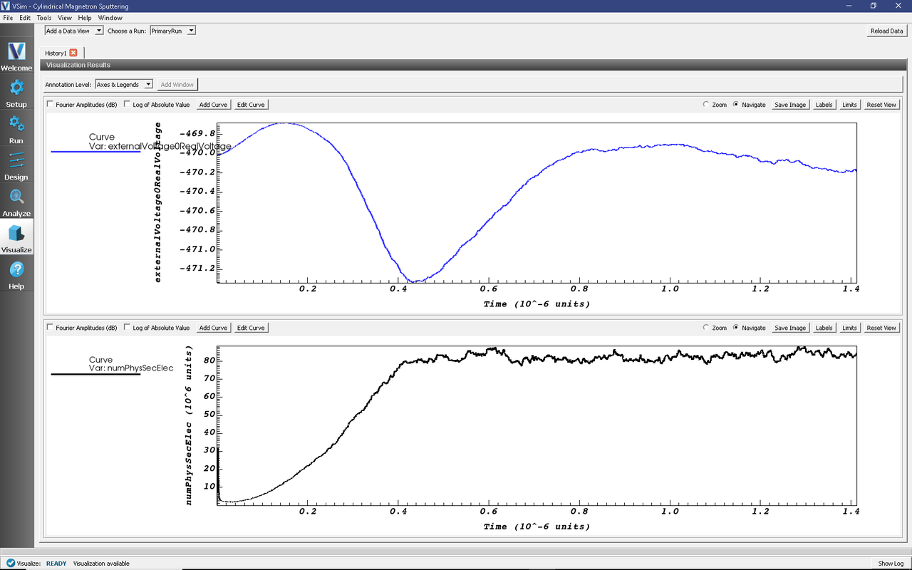
Fig. 640 The cathode potential (top) and number of physical secondary electrons (bottom) as a function of time.

These two history data sets are how we determine if the simulation has reached steady state. After the simulation has reached steady state at about 1 microsecond, the number of physical secondary electrons and the cathode potential are nearly constant.

The next data set we visualize is the self-consistent potential with the secondary electrons superimposed. To plot any field data with particle data superimposed, the user must first plot the field data, then the particle data. Follow these steps to view both of these data sets. If the data are already plotted you can skip these steps. However, these steps are applicable to lots of data types, so following these steps will allow you to view other data sets:

• Left-click on the “Add a Data View” option in the upper left corner and select “Data OverView”. This will open a new tab

• In the new tab expand the “Scalar Data” option and select Phi

• Slide the bar to the right at the bottom to view the potential and notice that the sheath thickness varies with time.

• Now expand the “Particle Data” option and expand “secElectrons” options. Check the box “secElectrons”

• You will now see the secElectrons macro particles plotted. To reduce the size of each particle, change the “Size” to 1

• Flip the axes by clicking on “Coord Swap” at the top of the window. This will plot the radial axis along the standard x-axis

• Finally, to preserve the aspect ratio, click the “Preserve Aspect Ratio” box at the top

The data are shown in Fig. 641.

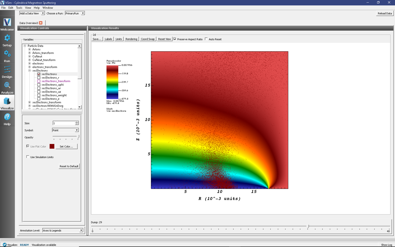
Fig. 641 Self-consistent potential with the secondary electrons superimposed.

Note that in VSim the state of your simulation is saved when you close a simulation. This means that all the visualization windows will re-open automatically when you re-load your simulation. However, the state that is saved might not be exactly what you first did. Therefore, you may need to re-swap the axes and you may need to unclick/re-click the particle data to visualize the particles.

One vital aspect to this problem is the presence of an external magnetic field which traps some population of electrons near the cathode. To view where the bulk of the secondary electrons form w.r.t. the external magnetic field, we next plot \(B_r\) with the secondary electrons superimposed. Follow similar steps to plotting the secondary electrons and the potential. This plot is shown in Fig. 642.

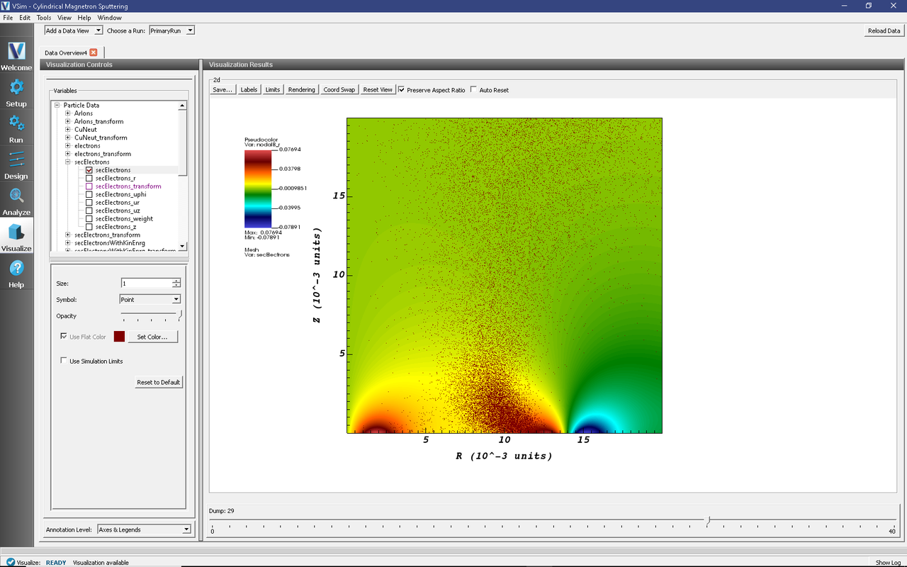
Fig. 642 Externally imposed magnetic field with the secondary electrons superimposed.

Finally, we plot copper density with the argon ions superimposed. This plot illustrates the main purpose of this simulation, which is the formation of Cu atoms that uniformly coat the surfaces in the chamber. To plot this data follow the previously discussed steps (recalling that field data must be plotted first). The copper density peaks where the ions are impacting the cathode the greatest. To visualize the data more easily we took two additional steps. (1) We changed the color scale of the copper density to range from \(10^{16}/\textrm{m}^3\) to \(2\times10^{21}/\textrm{m}^3\). We then plotted the data on a log scale. (2) We change the Z-axis to extend from 0 to 5 mm. The plot of copper density with ions superimposed is shown in Fig. 643.

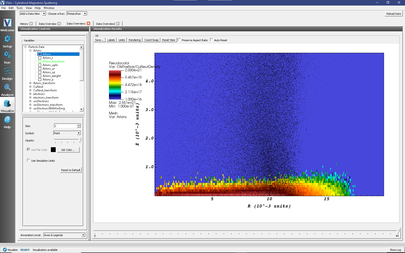
Fig. 643 The copper density plotted as a color contour plot with the Ar ions superimposed.

There are countless diagnostics that can be computed in VSim using analyzers already built. There are also numerous ways to visualize the data. If you have any further questions regarding this example (or any other example), data visualization in VSim or you need a custom analyzer for your application please contact Tech-X

Further Experiments

This problem involves a complex interaction of sources (secondary emission off of the cathode and ionization collision) and sinks at both the anode and cathode. Furthermore, the magnetic field profile and strength plays a key role in trapping just enough electrons to form a sheath but not too many electrons that then create a cascade of more secondary electrons. There are several parameters the user can change to determine the role of these various parameters in forming the sheath. For example, the user could try a different magnetic field (which the user has to provide). The user could also change the neutral density, the initial cathode voltage, and/or the external circuit parameters. Finally, the user could add more reactions to improve the physics of this example. Remember that one goal to try to maintain physically reasonable results is to reach steady state.