Turner Low Pressure Benchmarks (Turner.sdf)

Keywords:

capacitively coupled plasma, CCP, discharge, steady state, Turner

Problem Description: Overview of the Turner benchmarks

The physics of a capacitively coupled low-temperature plasma discharge can be quite complex. Sustainment of such a discharge involves a balance between multiple physical effects - losses of charged particles to the chamber walls, production of charged particles via ionizing collisions, and the formation of plasma sheaths (in response to disparate ion and electron mobilities) which mitigate both particle loss and production processes. Accurate numerical models of a capacitively coupled plasma discharge must capture physics associated with:

• Electron-neutral collisions (elastic/ inelastic/ ionizing)

• Ion-neutral collisions (isotropic/ backscattered)

• Particle loss, sheath formation, and imposed voltages at conducting surfaces

• Electrostatic potentials (from existing charge densities and boundary conditions)

• Electric fields (from potential gradients) and responsive charged particle motion

Inaccurate numerical predictions will be made by a particle-in-cell code which cannot accurately represent these basic processes. Even if the inaccuracy is small, its effect on the steady-state properties of the discharge can be significant.

In a notable paper published by M. M. Turner et al. [TDD+13] in 2013, modeling benchmarks for capacitively coupled plasmas were proposed which exercise each of the physics capabilities listed above. Turner’s paper documents the successful benchmarking of five independently developed particle-in-cell codes (not including VSim) in modeling low-temperature capacitively coupled plasma discharges at four different background pressures. A set of ‘accepted results’ for the steady-state ion density produced by the discharge, reproducible to within a specified, statistically-rigorous error tolerance by each of the five codes considered, is provided for each of the four cases. Numerical parameters for each case (e.g. sizes of discrete timesteps or finite grid cells) are also specified, with sufficient detail provided that other numerical models can attempt to reproduce the accepted results for each case to within the specified tolerance. VSim has been run for each of Turner’s cases in an effort to make such comparisons; in this example we will demonstrate various results from this modeling. Case 1 will be discussed extensively, and will be shown to pass Turner’s rigorous statistical benchmark. An explanation of how to reconfigure this example input file to run Turner’s Cases 2-4 will also be provided.

It should be noted that the modeling of physical plasma discharges is in fact not the objective of Turner’s work; no comparisons of Turner’s ‘accepted results’ with experimental data are ever made. Rather, the goal is to establish basic standards for codes that will model low-temperature plasma discharges. Agreement with the Turner benchmarks does not guarantee a code’s fitness for modeling arbitrary plasma discharges. It does, however, ensure that basic features of that code - e.g. its ability to push charged particles in response to electric fields, to determine the electrostatic potential from a given charge distribution, and to model charged-particle collisions with neutral atoms - are consistent with accepted practices, and that this consistency persists over a broad range of discharge parameters. At the end of this example we will discuss ways in which these simulations could be modified to more closely align with physical plasma discharges.

Problem Description: Physical description of Turner’s Case 1

In Turner’s Case 1, a capacitively coupled plasma discharge is sustained via a balance between collisional processes (source) and wall losses (sink). A one-dimensional box of length 6.7 cm contains neutral helium gas at room temperature (300 K) and density \(9.64 \times 10^{20}/m^{3}\) (30 mTorr of pressure at that temperature). The helium gas is weakly ionized, resulting in a population of free electrons and singly ionized helium atoms initially at density \(2.56 \times 10^{14}/m^{3}\). Initially, the helium ions are assumed to be at room temperature, while the free electrons are assumed to be considerably hotter (30,000 K). The left wall of the box is grounded, while the right wall oscillates with a bias voltage of 450 V at frequency 13.56 MHz. The oscillating voltage drive rapidly shifts the free electrons back and forth in the domain, but has little direct effect on the ions since their large mass leads to slow response times (much longer than the oscillation period).

Charged particles are lost upon collision with either the left or right wall, and are replenished by ionization of the background neutral gas by the hot electrons. These ionizing collisions repopulate both the electrons and helium ions in the plasma; the background neutral gas is treated as an infinite source. Plasma sheaths form near the walls, containing electric fields which are strong relative to those elsewhere in the plasma, and the particle density profiles adjust in response to the fields in the sheath. The sheath transit time, for ions, is much longer than the period of the oscillating potential; thus, multiple RF cycles occur while an ion crosses the sheath.

A quasi-steady state is attained when the loss rate of particles to the wall comes into balance with the ionization rate for a particular density profile shape. For ions, this density profile is essentially static in time; it is also highly sensitive to the physics of the discharge. Collisional processes represent an effective friction which impedes the outward transport of charged particles within the discharge, and even minor alterations to collision rates or scattering angles will locally modify these frictional forces to yield reshaped density profiles. Details associated with the underlying numerical implementation of individual collisional processes - e.g. the degree to which two-body elastic scattering in the center-of-mass frame is isotropic - thus also influence the steady-state solution.

This simulation can be performed with a VSimPD license.

Opening the Simulation

The Turner example is accessed from within VSimComposer by the following actions:

• Select the New → From Example… menu item from the File menu.

• In the resulting Examples window expand the VSim for Plasma Discharges option.

• Expand the Capacitively Coupled Plasmas option.

• Select Turner and press the Choose button.

• In the resulting dialog, create a New Folder if desired, and press the Save button to create a copy of this example.

All of the properties and values that create the simulation are now available in the Setup Window as shown in Fig. 510.

Fig. 510 Setup window for the 1D Turner example.

Modifying the Simulation: Turner’s Cases 2-4

This VSim example models Turner’s Case 1. If desired, VSim users can modify the example input file to instead model other cases in Turner’s benchmark paper. Users should be aware of the computational resources that will be needed to run each case and make comparisons with Turner’s benchmark data; the required resources are summarized in Computational Resources Needed For Turner Cases. Case 1 (this example) can be run to completion in approximately 8 core-hours (e.g. 8 hours in serial, or in about 30 minutes on a 16-core linux cluster). The higher neutral gas pressures used for the other Turner cases lead to shorter collisional mean free paths, and thus increase both the spatial and temporal resolution requirements of the simulations.

Computational resource requirements for Cases 3-4 are substantial. Tech-X strongly recommends the use of a parallel computing cluster (minimum 32 cores) for users who wish to run these cases.

Table 6 Computational Resources Needed For Turner Cases

	Neutral Pressure (Torr)	Computing Resources (core-hours)
Case 1	0.03	~8
Case 2	0.1	~170
Case 3	0.3	~750
Case 4	1.0	~4700

To change the example input file to model a different Turner case, users will need to adjust the following simulation parameters in the input file from the Case 1 defaults:

Table 7 Input Parameters For Turner Cases 1-4

	Case 1	Case 2	Case 3	Case 4
DT	RF_PERIOD/400.0	RF_PERIOD/800.0	RF_PERIOD/1600.0	RF_PERIOD/3200.0
NEUTRALN	9.64e20	3.21e21	9.64e21	3.21e22
RF_VOLTAGE	450.0	200.0	150.0	120.0
NX	128	256	512	512
PPC	512.0	256.0	128.0	64.0
NDENS	2.56e14	5.12e14	5.12e14	3.84e14
NSTEPS	512000	4096000	8192000	49152000

The number of simulation dumpfiles that will be created for each case, when run with these parameters, is as follows:

Table 8 Number of dumpfiles created

	Case 1	Case 2	Case 3	Case 4
Number of dumpfiles	125	1,000	2,000	12,000

The Turner examples proceed by first running the discharge out to steady-state, and then restarting the simulation (using a more frequent dump periodicity) to statistically sample the properties of this steady-state. The restart/sampling procedure will be explained below, and will use the data from the Number of dumpfiles created table.

Running the Simulation: Getting to Steady-State

After choosing which of Turner’s cases we will run, and making any needed changes to the input file, we are ready to run the simulation. This is done as follows:

• Proceed to the Run Window by pressing the Run button in the left column of buttons.

• Select the ‘Run Mode’ drop down menu and change it to parallel.

• Set ‘Number of Processes’ corresponding to your VSim license, shown above as the ‘Licensed Cores’.

• To run the file, click on the Run button in the upper left corner of the window. You will see the output of the run in the right pane. The run has completed when you see the output, “Engine completed successfully.” A snapshot of the simulation run during execution is shown in Fig. 511.

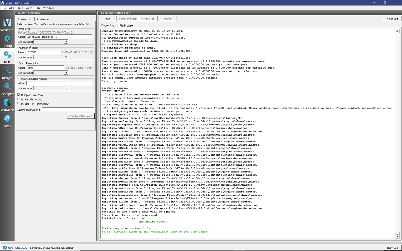
Fig. 511 Run window for the Turner example. Simulation runtime will depend on the number of cores available and on which of the Turner cases the user chooses to run (higher pressures yield longer runtimes).

Visualizing the Results: Basic Simulation Output

After the simulation has completed, we should quickly check to verify that the discharge has come to steady-state (at least to the degree that visual inspection permits; we will carry out more detailed mathematical/statistical analysis of the steady-state later in the example). To do so, click the Visualize button beneath the Run and Analyze buttons in the leftmost pane.

After a moment the visualization options for this data should appear.

We are going to look at a very basic metric for steady-state - is the number of simulation macroparticles for each species in the discharge both (a) nonzero, and (b) roughly constant in time? To do so, we will plot a time history of the macroparticle population of each species. This is done as follows:

• In the Visualization window, click the Add a data view → History menu. This will open a History tab.

• In the History tab, click on the Add Curve button. In the dropdown menu that appears (listing various 1D time histories that one might plot), select NumElec and then OK. A plot showing the variation of the electron macroparticle population in time should appear in the window.

• Click on the Add Curve button again, and this time select NumIons in the dropdown menu, and then OK. Another plot (of ion macroparticle population) should appear in the same window.

• Though it may already be apparent, we can adjust the y-axis limits to more convincingly show that the species macroparticle populations are both nonzero and approximately constant. To do so, click the Limits button, and adjust the Y-Axis range to be [0,25000].

From the resulting plot (also shown in Fig. 512), we can see that both the electron population and the (slightly higher) ion population have come to a nontrivial steady state. It is also reassuring that the average ion macroparticle population is higher than the average electron macroparticle population (given that the number of physical particles in a macroparticle is the same for both ions and electrons in this example). The higher mobility of the electrons allows them to be more easily lost at the simulation outset, and the formation of plasma sheaths is a direct consequence of the ensuing charge imbalance.

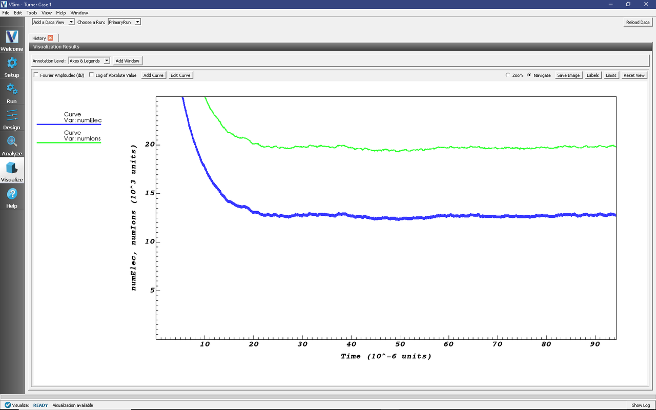
Fig. 512 Visualization window for the Turner example, demonstrating that the simulation has come to a nontrivial steady state.

As an exercise in using the Visualization window capabilities, users might demonstrate these same results by plotting the number of physical particles of each species, rather than the number of macroparticles. The new plot could be made in a separate window (use the Add Window button), or by deleting curves from the existing window (using the Edit Curve button) and thereafter adding new ones. The approximate Turner Case 1 steady-state values for ions and electrons are \(5.1 \times 10^{12}/m^{3}\) and \(3.2 \times 10^{12}/m^{3}\) respectively.

Running the Simulation: Sampling the Steady-State

Now that we have reasonable confidence that a steady-state discharge has been achieved, we will need to sample the properties of the steady-state. To do so, return to the Run window by clicking the Run button in the leftmost pane.

We will be restarting the simulation using a more frequent dump periodicity to sample the properties of the steady-state. In this manner we generate the data needed for the mathematical/statistical steady-state analysis.

The Restart Parameters table contains the parameters needed for the restart.

Table 9 Restart Parameters

	Case 1	Case 2	Case 3	Case 4
Number of Steps	13200	26400	52800	105600
Dump Periodicity	12	24	48	96
Restart at Dump Number	125	1000	2000	12000
Total Number of Dumps	1225	2100	3100	13100

Conceptually, we will be restarting the simulation from the final (presumably steady-state) dumpfile generated in the initial run (which is why the last entry of Restart Parameters has a corresponding entry in Number of dumpfiles created.) We will run the restarted simulation for 33 RF periods, and will sample the properties of the steady state every 0.03 RF periods. In this manner we obtain 11 datapoints at each fractional phase (T/100) of the RF period, yielding 1100 datapoints altogether (1100 dumpfiles are generated in the restart/sampling run). We will average over these datapoints to determine the properties of the steady state.

[Note: this averaging/sampling procedure is slightly different than the averaging procedure described in Turner’s paper. In that approach, very large quantities of data are generated since every timestep in a 32-period sequence is sampled. We have compared the two approaches and determined that the results are comparable; to use Turner’s procedure, one would set the Dump Periodicity of the restart run to 1, and modify the Number of Steps parameter to run over 32 RF periods instead of 33. Subsequent analysis would then need to take into account the much larger number of dumpfiles that will ensue.]

To restart the simulation and carry out the necessary sampling, do the following in the Run window:

• Change the Number of Steps value to match the value in the Restart Parameters table corresponding to the Turner case you are doing.

• In the Run window, change the Dump Periodicity value to match the value in the Restart Parameters table corresponding to the Turner case you are doing.

• In the Run window, change the Restart at Dump Number value to match the value in the Restart Parameters table corresponding to the Turner case you are doing.

• To run the file, click on the Run button in the upper left corner of the window. You will see the output of the run in the right pane. The run has completed when you see the output, “Engine completed successfully.”

A brief discussion of Turner’s chi-squared statistical metric

For each of Turner’s benchmark cases, a metric for agreement with the predicted physics results (in a statistical sense) has been provided. This statistical metric is based on the time-averaged ion density profile (a slowly-evolving quantity which is quite stable in steady-state) and takes the form \(\chi^{2} = \sum_{j=0}^{NX} {(n_{j} - \bar{n}_{j})^{2} \over \sigma_{j}^{2}}\). In this expression, \(n_{j}\) is the time-averaged ion density at the \(j\)-th gridpoint in the simulation and will be computed from the VSim data produced in the restart/sampling phase of this example. The expressions \(\bar{n}_{j}\) and \(\sigma_{j}\) are (respectively) Turner’s prediction for the time-averaged ion density at the \(j\)-th gridpoint, and a statistically computed population standard deviation for \(\bar{n}_{j}\) at this point. The simulation is assumed to have NX grid cells (the number of grid cells for each Turner case is listed in Input Parameters For Turner Cases 1-4) and thus has \(NX+1\) gridpoints; the uniform grid spacing is \(\Delta x = LX/NX\).

Heuristically, a VSim prediction for \(n_{j}\) at a given point that is less than one standard deviation \(\sigma_{j}\) away from Turner’s predicted value \(\bar{n}_{j}\) at that point will contribute only negligibly to the \(\chi^{2}\) sum; the contribution of this term to the sum will always be less than unity. VSim predictions that deviate from Turner’s predicted values by more than one standard deviation will contribute much more significantly to the sum. The expected values of \(\chi^{2}\) given by Turner for each case are:

Table 10 Expected Chi-Squared Values

	Case 1	Case 2	Case 3	Case 4
95%	55-303	177-435	405-693	417-665
99%	48-405	160-548	382-798	392-730

For a given case, Expected Chi-Squared Values asserts that if VSim is statistically indistinguishable from the five codes used in Turner’s benchmark, then the value of \(\chi^{2}\) computed from VSim data will fall within the 95% range with 95% probability (no more than one simulation in 20 should fall outside this range). Likewise, the value of \(\chi^{2}\) will fall within the 99% range with 99% probability (no more than one simulation in 100 should fall outside this range). When VSim predictions fall consistently within the ranges specified by Turner, we can have confidence in its predictive value for the case considered - at least, we can have confidence that it is capturing physics identical to the physics used by the other five codes in the benchmark.

In the following section we will use a VSim analyzer to compute the value of \(\chi^{2}\) for the run we have just completed.

Analyzing the Results: Comparing with Turner chi-squared diagnostic

To determine whether VSim has statistically matched the Turner benchmark, return to the VSim analysis window by clicking on the Analyze tab in the leftmost pane.

In the list of available analyzers, find and select computeTurnerChi.py. A window should appear at right showing the default input parameters for this analyzer. The case option allows users to switch between Turner’s cases 1, 2, 3, or 4. If this parameter is changed, the user should also change the start_dump and end_dump options to be consistent with the data in the Restart Parameters table. The correct start_dump option is obtained by adding 1 to the Restart at Dump Number value found in the table, for the Turner case under consideration. The correct end_dump option is the same as the Total Number of Dumps option in the table, for the Turner case under consideration.

Clicking the Analyze button computes a time-averaged value for \(\chi^{2}\) using all dump files in the interval start_dump to end_dump. Output for this analyzer is shown in Fig. 513; for this particular run, a value of \(\chi^{2} = 96.16\) was obtained. This number should be compared with the ranges for Case 1 shown in Expected Chi-Squared Values.

For this run, the computed \(\chi^{2}\) value falls within both the 95% and 99% allowable ranges of the Expected Chi-Squared Values table for Turner’s Case 1. The value of \(\chi^{2}\) will almost certainly differ when this example is run on other computing platforms, or even when this example is repeated on the same platform; users should not be alarmed if their values do not precisely match the values shown here. Nevertheless, statistical agreement with Turner’s benchmark can be claimed if the computed \(\chi^{2}\) values deviate from Turner’s 95% range no more often than one run in twenty (on average), or from Turner’s 99% range no more often than one run in a hundred (on average). This result should be independent of computing platform.

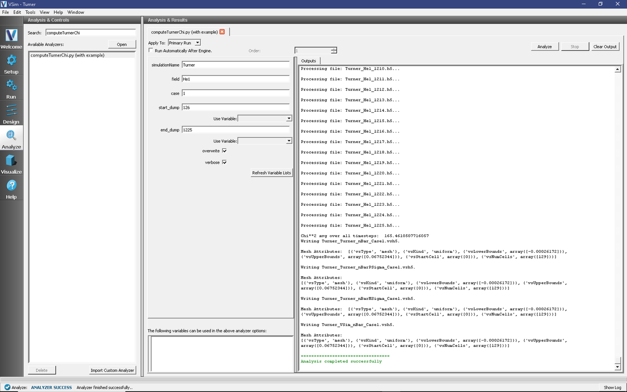
Fig. 513 Analysis window for the Turner example, showing input parameters for, and output from, the computeTurnerChi.py analyzer for Turner’s Case 1. The computed value for \(\chi^{2}\) falls within Turner’s predicted ranges, indicating that these VSim results are statistically indistinguishable from those generated by the five other codes used in the benchmark.

Analyzing the Results: Comparing with Turner electron energy distribution function

In this section, we will construct an electron energy distribution function (EEDF) from our steady-state simulation data. Afterwards, we will compare this function to the EEDF predicted by Turner.

Return to the VSim analysis window by clicking on the Analyze tab in the leftmost VSim Composer pane. Then, double-click on the computeTurnerEEDF.py analyzer in the list of available analyzers on the left of the window. A window should appear showing the default input parameters for this analyzer.

This analyzer operates on the macroparticle data which VSim periodically dumps. Given a macroparticle dumpfile corresponding to a particular time in the simulation, one can extract from this file a histogram of the particle energies at that time. Because the Turner discharges are periodic, the distribution of particle energies will varies slightly in time based on the phase of the periodic driving voltage, so we will need to sample over a sequence of dumpfiles which sample the EEDF uniformly in the different phases. This is done in just the same manner as we sampled other properties of the steady-state above; we will use the same start_dump and end_dump values for the analyzer as we did for the computeTurnerChi.py analyzer above. In doing so, we will sample the EEDF associated with the steady-state discharge. The default start_dump and end_dump values assume that files from Turner’s Case 1 are being analyzed using the less data-intensive sampling method described previously.

The analyzer constructs a normalized histogram \([\epsilon,f(\epsilon)]\) of particle energies, with energy given in units of electron-volts, for all particles within the specified range of dumpfiles. The normalization follows that of Turner; we require that \(\int_{0}^{\infty} \sqrt{\epsilon} f(\epsilon) d\epsilon = 1\) for the desired distribution \(f(\epsilon)\).

After adjusting the start_dump and end_dump values (if needed), click on the Analyze button at the top of the right panel to run this analyzer.

When the analyzer is finished, it will display the histogram bins and the histogram data in the log window at right, and report that the “Analysis completed successfully”. For large datasets (such as the one we will construct), only abbreviated representations of the bin and the data arrays will be shown. Representative output for the analyzer, together with its default input parameters, is shown in Fig. 514.

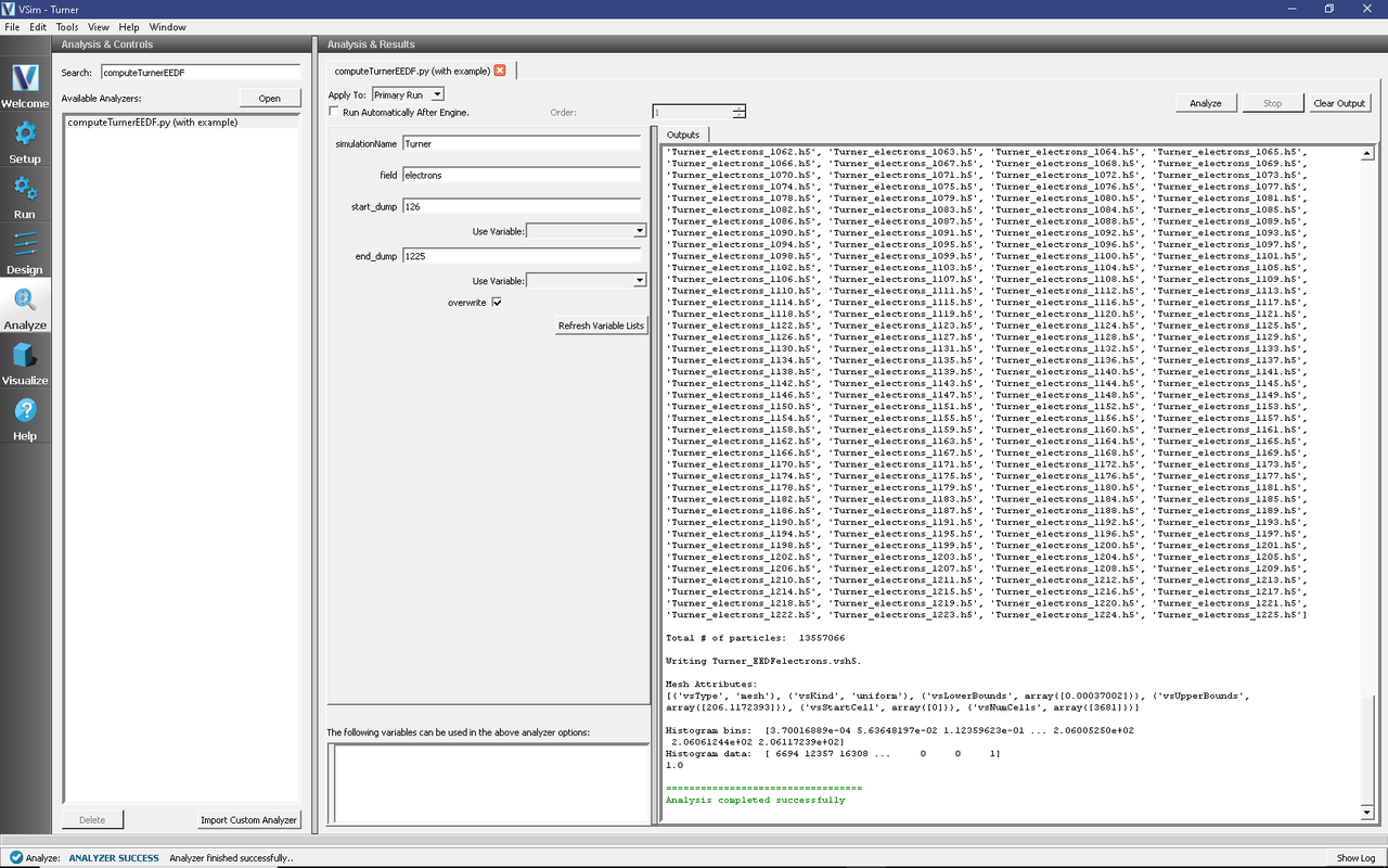
Fig. 514 Analysis window for the Turner example, showing input parameters for, and output from, the computeTurnerEEDF.py analyzer for Turner’s Case 1.

The analyzer output is written to a file Turner1_EEDFelectrons.vsh5 which contains the full bin and data arrays (normalized) of the computed histogram. This file can be viewed in the Visualize window, which we will now do.

Visualizing the Results: Comparing with Turner electron energy distribution function

Return to the VSim visualization window by clicking on the Visualize tab in the leftmost VSim Composer pane.

The histogram plotted in the previous section is a 1D plot of probability as a function of energy. To view it, click the Add a Data View tab in the top left of the visualization window, and select 1-D Fields. A new tab with this designation will open in the window below.

Click the Add Curve button in the plot window. From the dropdown menu that appears, select the electrons_EEDF variable and click OK. A plot should appear in the window.

We will be comparing with Figure 6 of Turner’s paper, which is plotted on a log-linear scale. To make our plot look like Turner’s plot, do the following:

• Switch the y-axis to a logarithmic scale by clicking the Log of Absolute Value checkbox at the top of the plot window.

• Change the plot limits by clicking the Limits box at the top right of the plot window. The X-Axis values should be changed to cover the range 0 (Min) to 60 (Max), while the Y-Axis values should be changed to cover the range -5 (Min) to -1 (Max). (On the logarithmic scale, these values represent the powers of ten spanned by the plot on the y-axis.)

The resulting plot is shown in Fig. 515, and can be compared with Figure 6 of Turner’s paper [TDD+13].

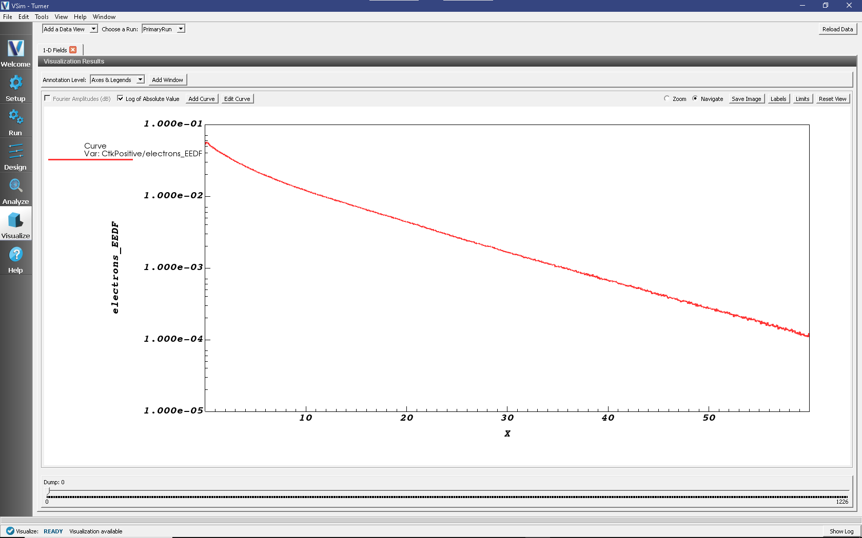
Fig. 515 Visualization window for the Turner example, showing a plot of the normalized steady-state electron energy distribution function for Turner’s Case 1. This plot can be compared with Figure 6 of Turner’s benchmark paper, noting that in that plot the EEDF distributions are normalized inconsistently from what the text indicates [a multiplicative factor of approximately 0.414 reduces the value of \(f(\epsilon)\) below the properly normalized VSim result].

Analyzing the Results: Comparing with Turner power deposition diagnostic

In this section, we will construct time-averaged power density profiles \(\langle {\bf E} \cdot {\bf J}_{\alpha} \rangle\) for each species (\(\alpha\) = electrons, ions). Thereafter, we will compare these profiles to the power density profiles predicted by Turner.

Return to the VSim analysis window by clicking on the Analyze tab in the leftmost VSim Composer pane. Then, double-click on the computeTurnerJdotE.py analyzer in the list of available analyzers on the left of the window. A window should appear showing the default input parameters for this analyzer.

This analyzer operates on the electric field profiles and species current density profiles which VSim periodically dumps. Although these are vector field quantities, for this example only the x-coordinate will be relevant. Electric field components in the ignored directions (y and z) are zero in this simulation.

The analyzer computes a time-averaged \(\langle {\bf E} \cdot {\bf J}_{electron} \rangle\) and \(\langle {\bf E} \cdot {\bf J}_{ion} \rangle\) using the same averaging procedure as was used to plot the EEDF above; it should use the same start_dump and end_dump values that were used in computeTurnerChi.py and computeTurnerEEDF.py above to sample the power density profiles associated with the steady-state discharge. The default start_dump and end_dump values for this analyzer assume that files from Turner’s Case 1 are being analyzed using the less data-intensive sampling method described previously.

After adjusting the start_dump and end_dump values (if needed), click on the Analyze button at the top of the right panel to run this analyzer.

When the analyzer is finished, it will display in the right-hand window the full arrays containing the computed power density profiles, in units of kiloWatt per cubic meter. The number of points in these arrays is equal to the number of grid cells for the particular Turner case chosen, i.e. the \(NX\) value in Input Parameters For Turner Cases 1-4. An “Analysis completed successfully” message should also appear in the log window at right.

Representative output for the analyzer, together with its default input parameters, is shown in Fig. 516.

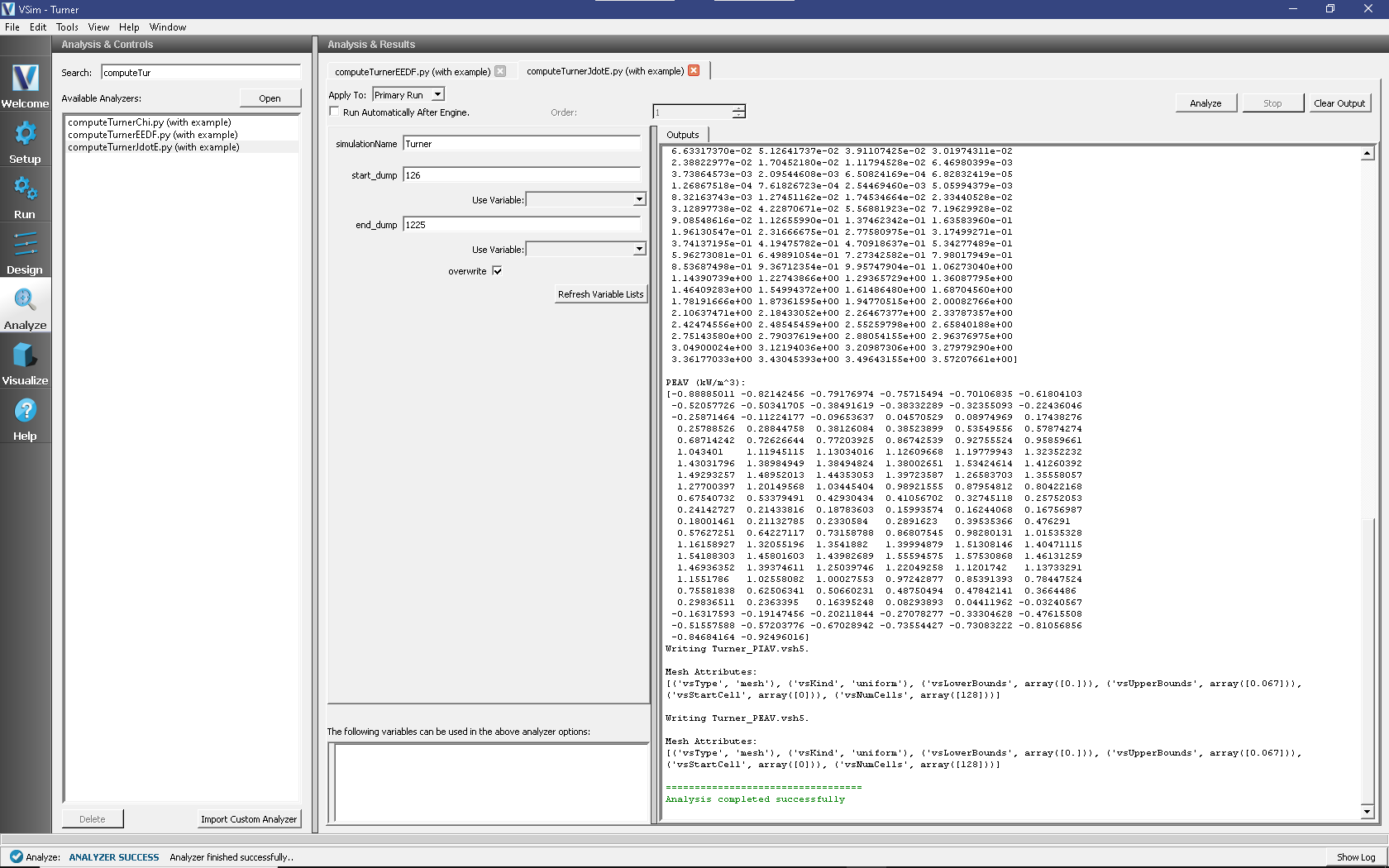
Fig. 516 Analysis window for the Turner example, showing input parameters for, and output from, the computeTurnerJdotE.py analyzer for Turner’s Case 1.

The analyzer output is written to two files, Turner1_PEAV.vsh5 and Turner1_PIAV.vsh5, which are respectively the electron and ion power density profiles averaged over the specified time interval. These files can be viewed in the Visualize window, which we will now do.

Visualizing the Results: Comparing with Turner power deposition diagnostic

Return to the VSim visualization window by clicking on the Visualize tab in the leftmost VSim Composer pane.

The power density profiles generated in the previous section are, like the EEDF, 1D plots that can be viewed from the 1-D Fields tab of the visualization window. You may need to click the Reload Data button at the top right of the window to enable these files to be seen in the window. Any existing plots in the 1-D Fields panel can be erased by clicking the Edit Curve button, and thereafter the Remove Selected Curve button.

We are going to look at the electron power density profile first. Click the Add Curve button in the plot window. From the dropdown menu that appears, select the PEAV variable and click OK. A plot should appear in the window.

We will be comparing this plot with Figure 4 of Turner’s paper. To make our plot look like Turner’s plot, change the plot limits by clicking the Limits box at the top right of the plot window. The X-Axis values should be changed to cover the range 0 (Min) to 0.067 (Max), and the Y-Axis values should be changed to cover the range -2 (Min) to 9 (Max). (Turner plots x/LX, with LX = 0.067 meters; we are plotting x directly in the range \([0,LX]\).)

The resulting plot is shown in Fig. 517; the data compares favorably with Figure 4 of Turner’s paper [TDD+13].

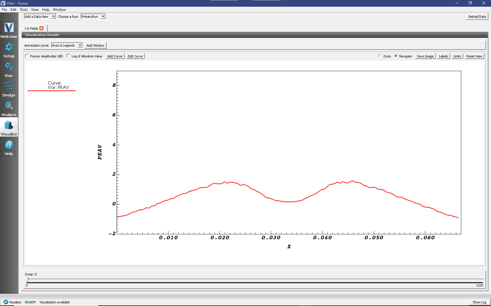
Fig. 517 Visualization window for the Turner example, showing a plot of the normalized steady-state electron power density profile for Turner’s Case 1. This plot can be compared with Figure 4 of Turner’s benchmark paper.

We will now look at the ion power density profile. Click the Edit Curve button, and thereafter the Remove Selected Curve button, to clear the electron power density profile plot. Then click the Add Curve button in the plot window. From the dropdown menu that appears, select the PIAV variable and click OK. A new plot should appear in the window.

We will be comparing this plot with Figure 5 of Turner’s paper. To make our plot look like Turner’s plot, change the plot limits by clicking the Limits box at the top right of the plot window. The X-Axis values should again be changed to cover the range 0 (Min) to 0.067 (Max), and the Y-Axis values should be changed to cover the range 0 (Min) to 4.5 (Max). (Again, Turner plots x/LX, with LX = 0.067 meters; we are plotting x directly in the range \([0,LX]\).)

The resulting plot is shown in Fig. 518, and the data compares favorably with Figure 5 of Turner’s paper [TDD+13].

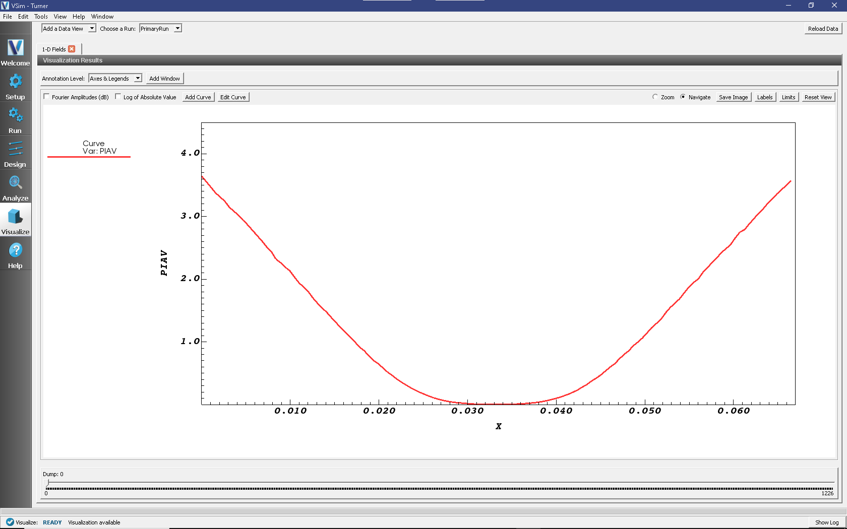
Fig. 518 Visualization window for the Turner example, showing a plot of the normalized steady-state ion power density profile for Turner’s Case 1. This plot can be compared with Figure 5 of Turner’s benchmark paper.

Further Experiments

As we have noted, the Turner benchmarks provide useful metrics for assessing whether or not basic features of a PIC-MCC code - its ability to push charged particles in response to electric fields, to determine the electrostatic potential from a given charge distribution, and to model charged-particle collisions with neutral atoms - are consistent with accepted practices. The benchmarks do not guarantee a code’s fitness for modeling arbitrary low-temperature plasma discharges, though the features listed above are certainly necessary for such modeling.

Nevertheless, given confidence in the benchmark model, one can then move toward a more physically representative model of a given plasma discharge by incrementally altering the benchmark file to include additional physics. Some alterations might be simple and require little additional verification; for example, Turner’s benchmark stipulates an electron mass of \(9.109 \times 10^{-31}\) kg (exactly), and equal ion and neutral masses of \(6.67 \times 10^{-27}\) kg (exactly). VSim’s underlying code infrastructure works the same way even if we adjust these values to include more significant digits, and/or to more carefully account for the mass difference between neutral and ionized helium atoms. No additional verification would be needed to make such a change, but the steady-state discharge profiles and the other plots we have made will change slightly due to the added physics. In a similar way, adding a new collision process to the discharge (using an appropriate cross-section data file, as documented in Obtaining Cross-Sections from LxCat) adds only additional physics processes to the discharge whose numerical implementation we trust.

Other alterations to the input file cannot rely directly on the consistency argument established by passing Turner’s benchmarks. Changes that alter the underlying physics of a particular collision, e.g. switching the electron-neutral ionization scattering type to VahediSurendra default instead of Turner, can no longer be checked against the collisional interaction physics of Turner’s model. While it is believed that the Vahedi-Surendra scattering model more closely approximates physical reality than the model used in the benchmark (and Tech-X further believes that this scattering model is implemented correctly in VSim, consistent with Ref. [VS95]), the new steady-state of the discharge cannot be compared with Turner’s directly. (In such cases, it may be of interest to the user to verify that the physics of the new collision process, as calculated by VSim, matches up with what the user expects. This could be done by constructing a reduced example that models only the new collision process; a modified version of the Townsend Discharge (townsend.sdf) example could work well for this purpose.)