2D Capacitive Plasma Chamber (capacitivelyCoupledPlasma2DT.pre)
Keywords:
- capacitively coupled plasma discharge under RF and DC voltage in 2D cylindrical system.
Problem description
The capacitively coupled plasma (CCP) is one of the most common types of industrial plasma sources. These plasma discharges typically take place between metal electrodes in a reaction chamber and are driven by a radio frequency (RF) or direct current (DC) power supply. The plasma is sustained by ohmic heating in the main body and stochastic heating through the capacitive sheath.
This example demonstrates the generation of a capacitively coupled plasma inside an axially symmetric reaction chamber with a 50 mm radius and 50 mm length. The top (\(r=0.050\) m) and right (\(z=0.050\) m) boundaries are grounded at zero potential. A target located at the bottom of the chamber (along the \(z=0\) boundary) is connected to a 60 MHz AC voltage source at 200 V. There is a small gap of 5 mm between the target and the grounded wall which is modeled via Neumann boundary conditions. The \(r=0\) boundary also invokes a floating potential using Neumann boundary conditions. The chamber is filled with a background gas of neutral Argon at about 0.005 Torr \(\left(2.0 \times 10^{20} \ \text{m}^{-3}\right)\). An initial spatially averaged electron and Ar+ density of \(5 \times 10^{11} \ \text{m}^{-3}\) is seeded to start the discharge. The particles are loaded with a density of \(5 \times 10^{11} \ \text{m}^{-3}\) every time step for the first 5000 time steps.
This simulation can be performed with a VSimPD license.
Opening the Simulation
The Capacitively Coupled Plasma 2D example is accessed from within VSimComposer by the following actions:
Select the New → From Example… menu item in the File menu.
In the resulting Examples window expand the VSim for Plasma Discharges option.
Expand the Capacitively Coupled Plasmas (text-based setup) option.
Select “2D Capacitive Plasma Chamber (text-based setup)” and press the Choose button.
In the resulting dialog, create a New Folder if desired, and press the Save button to create a copy of this example.
The basic variables of this problem should now be alterable via the text boxes in the left pane of the Setup Window, as shown in figure Fig. 519.
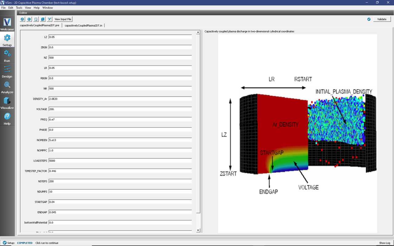
Fig. 519 Setup Window for the Capacitively Coupled Plasma 2D example.
Input File Features
The self-consistent electric field is solved from Poisson’s equation by an electrostatic solver in cylindrical coordinates. Time-dependent Dirichlet boundary conditions are used to set up the boundaries of electric fields around the reaction chamber walls.
The plasma is simulated with macroparticles which are moved using the Boris pusher in cylindrical coordinates. Various types of elastic and inelastic collisions of the particles are calculated.
The Setup Window has various parameters available for easy manipulation including the density of the argon background gas (DENSITY_Ar), the voltage (VOLTAGE), and the frequency (FREQ).
Running the simulation
Once finished with the problem setup, continue as follows:
Proceed to the Run Window by clicking the Run button in the left column of buttons.
Choose your desired parallel computing options under Run Mode.
To run the file, click on the Run button in the upper left corner of the Logs and Output Files pane. You will see the output of the run in that pane. The run has completed when you see the output, “Engine completed successfully.” This is shown in Fig. 520.
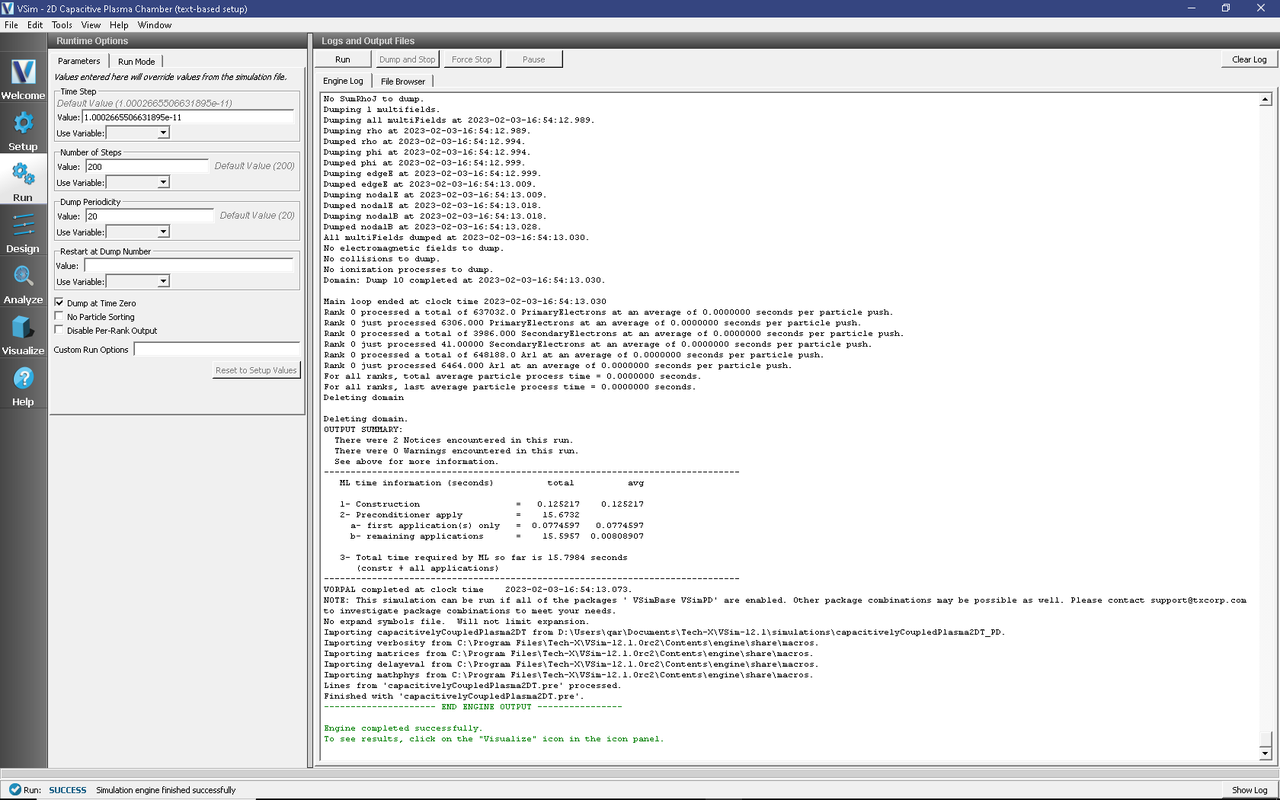
Fig. 520 The Run Window at the end of execution.
Visualizing the results
After performing the above actions, continue as follows:
Proceed to the Visualize Window by clicking the Visualize button in the left column of buttons.
To plot the potential:
In the Visualization Controls pane, click on the Data Overview tab and expand Scalar Data
Select phi
Move the dump slider at the bottom of the Visualization Results pane to the right to move forward in time.
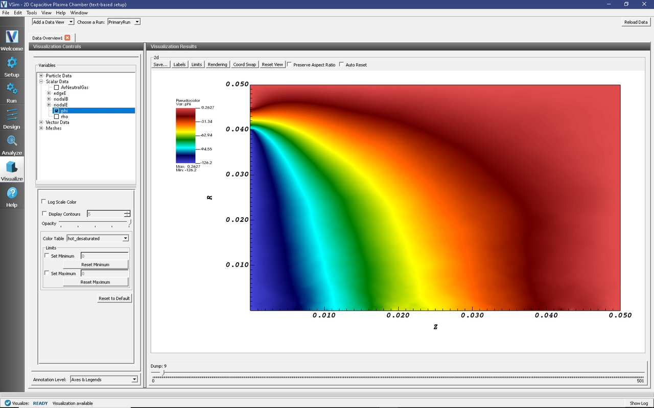
Fig. 521 Visualization of the electric potential in \(r\)-\(z\) coordinates.
Further Experiments
With a time-step of \(10^{-11}\) seconds, running this simulation for the default 200 time-steps will only capture part of the first oscillation. With the frequency set to \(6\times 10^7\) Hz, the oscillation period is \(1.667\times 10^{-8}\) seconds, which corresponds to 1,667 time-steps. To see the approximate steady-state behavior of this example, set the number of time-steps to 10,000 or more and restart or re-run the simulation. When running in parallel on 4 processors, this should take approximately two hours to complete.
After \(5\times 10^{-8}\) seconds, or 5000 dumps, the plasma sheath starts to exhibit oscillating steady-state behavior. To view the behavior of the oscillating plasma sheath, take the following steps:
In the Data Overview tab, expand Scalar Data
Select rho
At the top of the Visualization Results pane, click Colors to open the Color Options window
Select “Fix Minimum” and set the minimum to
-0.0005, then select “Fix Maximum” and set the Maximum to0.0005(or experiment with minimum and maximum values for best results) and click OKMove the dump slider at the bottom of the Visualization Results pane to dump 250.
After 250 time-steps, the plasma density should appear as shown in Fig. 522. The green areas at approximately zero charge density denote the quasi-neutral plasma bulk, while the red areas (positive charge density) denote the non-neutral plasma sheath.
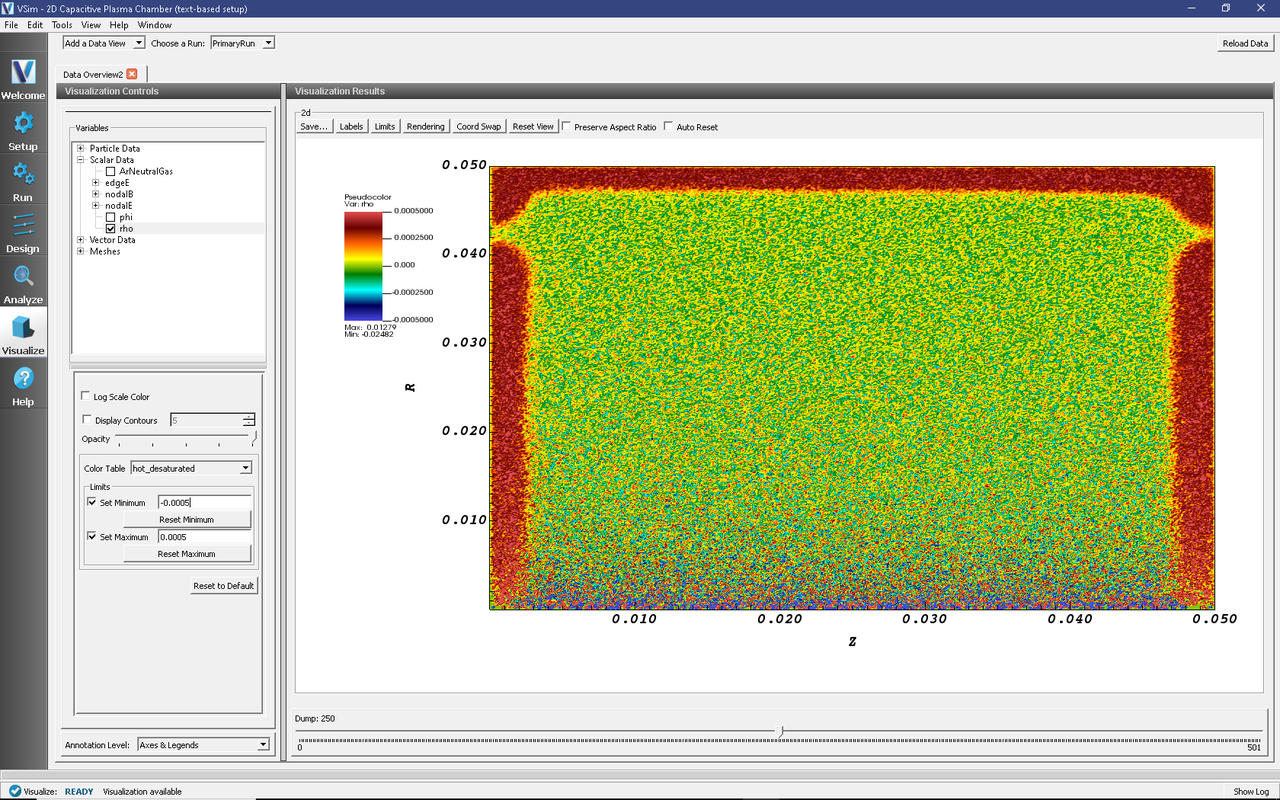
Fig. 522 Visualization of the plasma sheath via the charge density.
To view the plasma sheath potential profile, take the following steps:
In the Visualize window, select Field Analysis from the Add a Data View drop-down menu
In the Field Analysis tab, click on the Fields drop-down menu and select phi
Under Lineout Settings click on the Horizontal tab, and change the intercept value if desired
Click Perform Lineout
The electric potential as well as the axial potential profile should now be visible as shown in Fig. 523. Move the slider to the right to see how the plasma sheath potential oscillates in time.
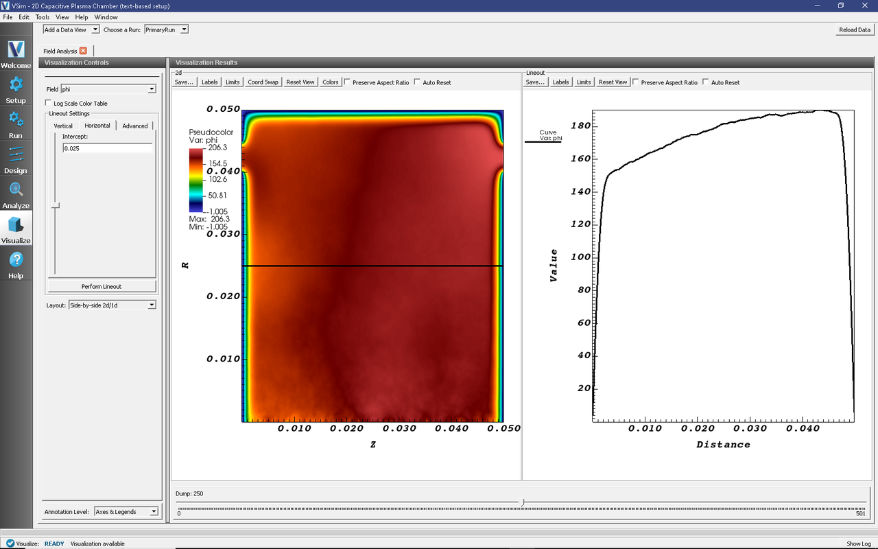
Fig. 523 Visualization of the plasma sheath via the charge density.