Antenna on Human Hand with Dielectric (antennaOnHand.sdf)

Problem Description

This problem calculates the far-field radiation pattern of a small (cellular mobile) antenna mounted on a small curved dielectric (plastic/PVC). The fields interact with the human hand for which the bone structure was approximated by long thin cylinders. The antenna feed is a 850 MHz source.

This simulation can be performed with a VSimEM license.

Opening the Simulation

The Antenna on Human Hand with Dielectric example is accessed from within VSimComposer by the following actions:

• Select the New → From Example… menu item in the File menu.
• In the resulting Examples window expand the VSim for Electromagnetics option.
• Expand the Antennas option.
• Select “Antenna on Human Hand with Dielectric” and press the Choose button.
• In the resulting dialog, create a new folder if desired, and press the Save button to create a copy of this example.

The Setup window is now shown with all the implemented physics and geometries. See Fig. 172.

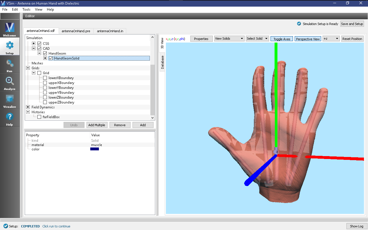
Fig. 172 Setup Window for the Antenna on Human Hand with Dielectric example, with Grid and farFieldBox History hidden.

Simulation Properties

This file allows the modification of antenna operating frequency, dimensions, orientation, and simulation domain size.

Running the Simulation

After performing the above actions, continue as follows:

• Proceed to the Run Window by pressing the Run button in the left column of buttons.
• To run the file, click on the Run button in the upper left corner of the Logs and Output Files pane. You will see the output of the run in that pane. The run has completed when you see the output, “Engine completed successfully.” This is shown in the window below.

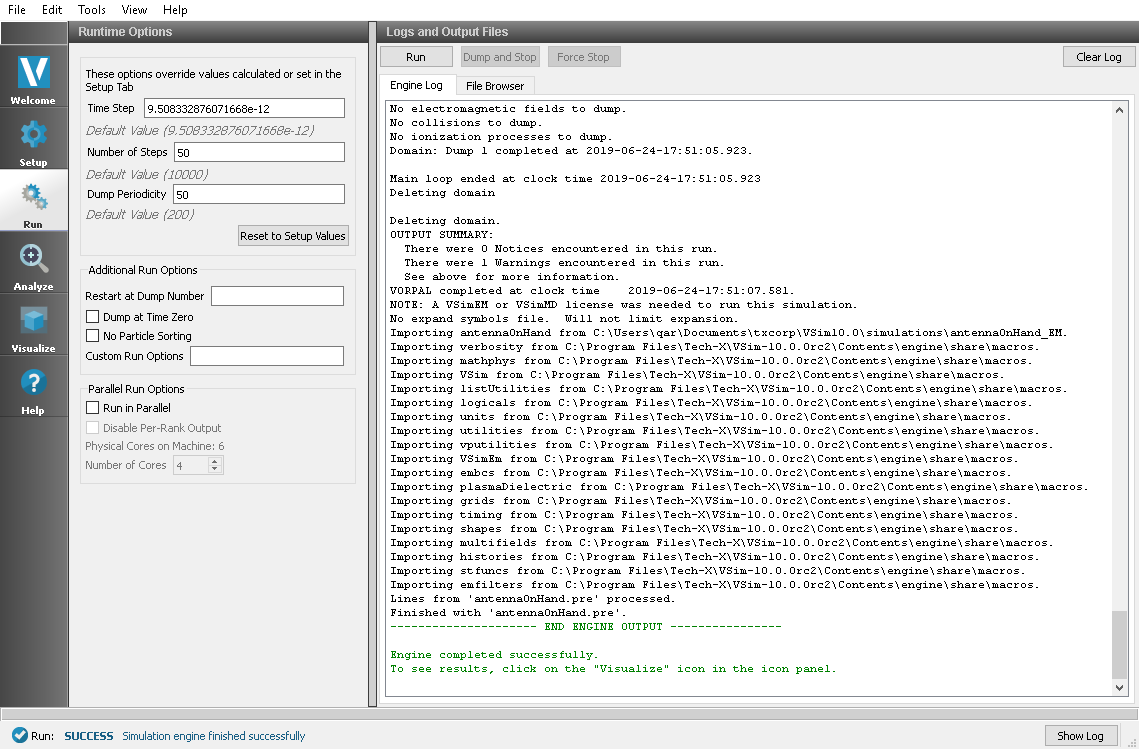
Fig. 173 The Run Window at the end of execution.

Analyzing the Results

After performing the above actions, continue as follows:

• Proceed to the Analysis window by pressing the Analyze button in the left column of buttons.
• Select computeFarFieldFromKirchhoffBox.py from the list and select “Open” (Fig. 174)
• Input values for the analyzer parameters. The analyzer may be run multiple times, allowing the user to experiment with different values.
  • simulationName - antennaOnHand (name of the input file)
  • fieldLabel - E (name of the electric field)
  • farFieldRadius - 0.5 (distance to far field in m, 10.0 is a good value)
  • timeStepStride - 150 (number of timesteps between far field calculations; determines how many far fields are output)
  • getFourierComponent - 0, do not integrate assuming single fourier frequency
  • frequency - not used because getFourierComponent is false
  • numTheta - 60 (number of theta points in the far field, 30 for a quick calculation, 60 for finer resolution)
  • numPhi - 120 (number of phi points in the far field, 60 for a quick calculation, 120 for finer resolution)
  • zeroThetaDirection - (0,0,1) (determines orientation of far field coordinate system)
  • zeroPhiDirection - (1,0,0) (determines orientation of far field coordinate system
  • varyingRadiusMesh - 1 (Set to 1 in order to make far field mesh adapt to magnitude of far field solution: the classic lobe view - Note: using a varying mesh option will make the analyzer run very slow.)
• Click “Analyze”
• Depending on the values of numTheta, numPhi, and timeStepStride, the script may need to run for several minutes or longer.

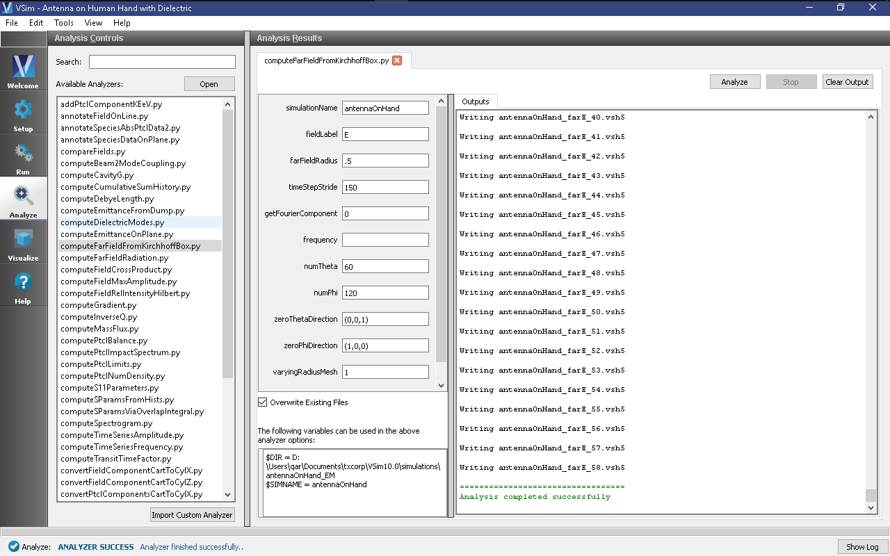
Fig. 174 The Analyze panel after running computeFarFieldFromKirchhoffBox.py.

Visualizing the Results

Proceed to the Visualize Window by pressing the Visualize button in the left column of buttons.

The far field radiation pattern can be found in the Scalar Data variables of the Data Overview tab. Expand farE and check the farE_Magnitude box. The poly_surface (HandGeomSolid) under Geometries, can also be plotted. Fig. 175 shows the visualization at last far-field time.

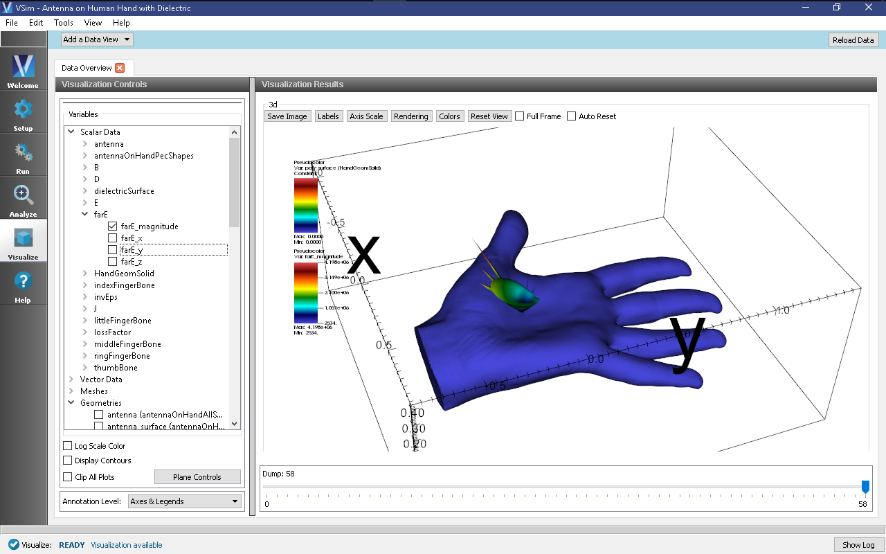
Fig. 175 The Far Field Radiation Pattern.

Further Experiments

The skin can be included as an additional geometry by simply importing the hand geometry a second time within the same set-up, but with a very slightly higher scaling factor and setting the Skin material for the hand geometry with the higher scaling factor. Some “by eye” adjustments of the x-, y-, and z- translation values may be needed.