Introduction to the Visualize Window
VSimComposer’s Visualization feature is a flexible and comprehensive model viewer based on VisIt. The simulation tutorials and examples in VSim Examples provide several examples of using the Visualization feature’s options in context.
The VSimComposer visualization tool is context sensitive, meaning that only those features that can be used with the current data are made available from the interface.
For more information on VisIt, please see: https://wci.llnl.gov/codes/visit/ and http://www.visitusers.org/index.php?title=VisIt_Wiki
For more information on using the VisIt context menu see: Tools/VSimComposer Menu: Visualization Options.
The Visualization window is divided into a Visualization Controls pane on the left and a Visualization Results pane on the right.
The type of data available to view is governed by the Data View pull down menu.
Select the Visualize Icon from the Icon Panel
Upon successful completion of the simulation run, the last message in the Engine Log tab is a reminder that you can now select the Visualize icon from the icon panel on the far left of the VSimComposer window as seen in Fig. 96.
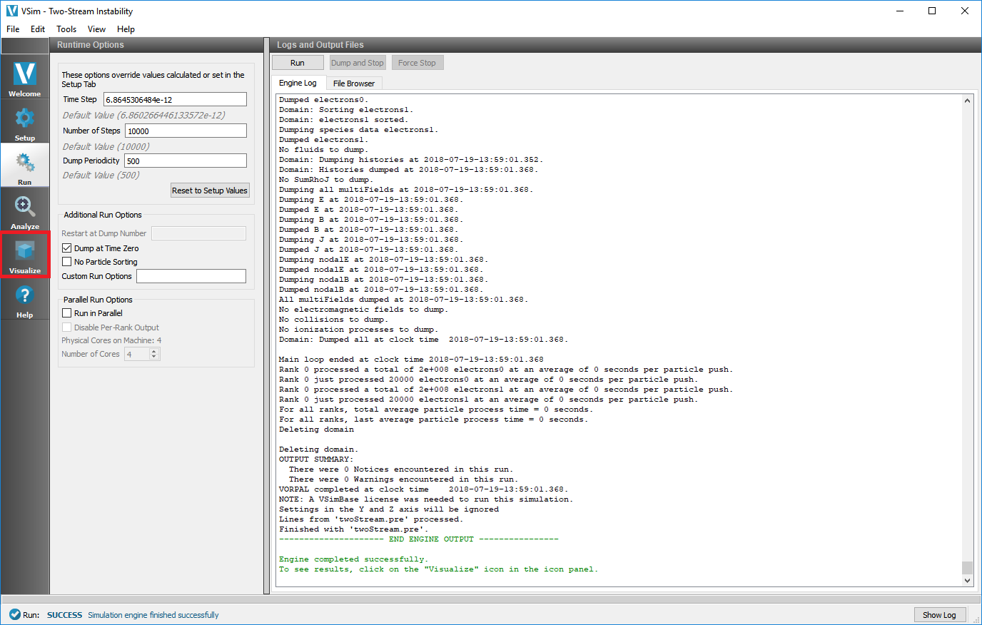
Fig. 96 Visualize Icon in Icon Panel
Data View Pull-down Menu
In the top left of the main pane, you may select the kind of analysis
that is to be performed. Again, this menu is context sensitive, so not
all options may be available for your simulation. For example, you may
only choose phase space if you have particles, and you may only paint
fields onto surfaces if you have complex boundaries specified in
GridBoundary blocks.
- Data Overview
- 1-D Fields
- Field Analysis
- History
- Phase Space
- Binning
- Paint Fields
See Fig. 97.
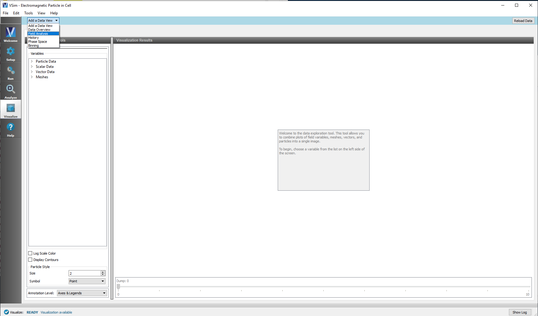
Fig. 97 Data View Menu
Standard Controls Available Across Multiple Views
Several control buttons or choices are available across several different Data Views. They have the same functionality in each case and are documented below.
Annotation Level
To adjust the Annotation Level, use the Annotation Level drop-down menu at the lower left of the Visualization Controls pane.
- No annotations
- Axes only
- Axes & Legends
- All annotations
See Fig. 98.
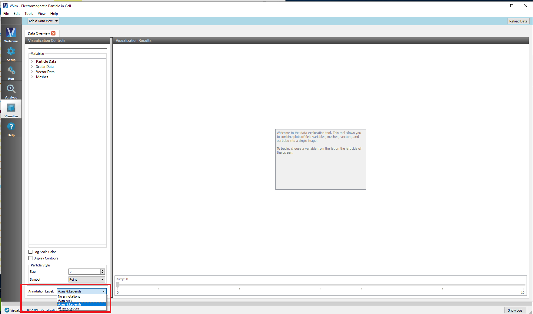
Fig. 98 Annotation Level
Reload Data
You can visualize data from a simulation run as soon as it becomes available. If you decide to visualize data before a run is complete by switching to the Visualize tab, the VSim engine continues creating data files in the background. Later, when more data is available for visualization or the simulation run is complete, use the Reload Data button in the top right-hand corner to visualize the new data. See Fig. 99.
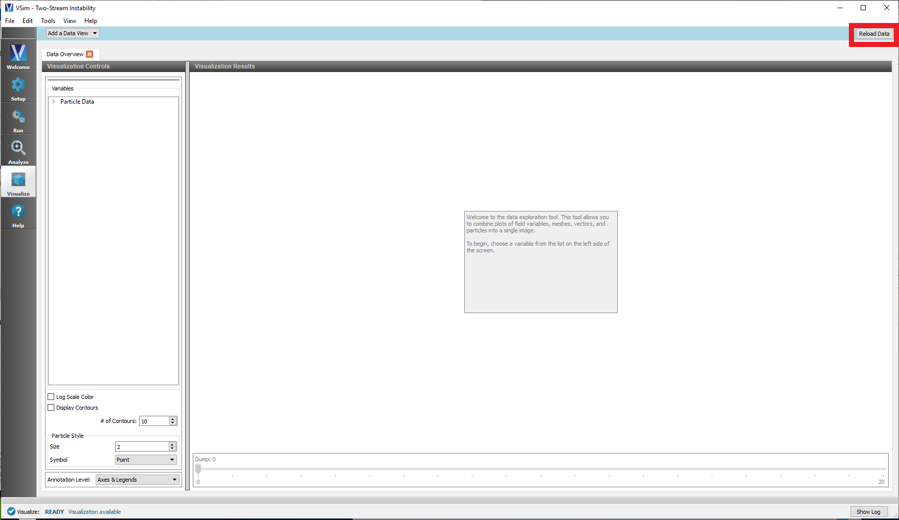
Fig. 99 Controls Pane Buttons
Save Image
This button saves the current image to your computer. You will be given options on where to save, the file name, and format as well as some options on size and dimension.
Labels
This brings up the Axis Labels window. See Fig. 100.
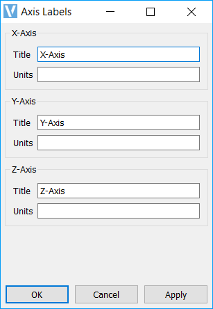
Fig. 100 Axis Labels Menu
Axis Scale
This button enables adjusting the Scaling Factor for each axis. See Fig. 101.
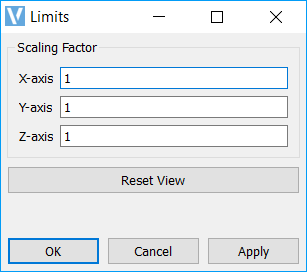
Fig. 101 Axis Scale Menu
Rendering
This button allows for adjustment of the lighting and stereo effects. See Fig. 102.
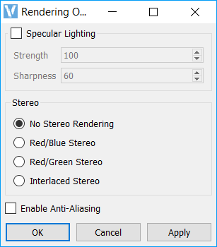
Fig. 102 Rendering Menu
Colors
This button allows changing of the color table used for the plot and allows you to set limits on the minimum and maximum. See Fig. 103.
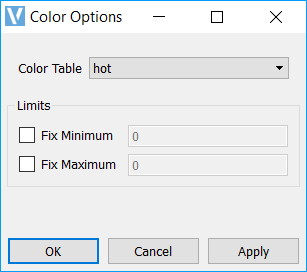
Fig. 103 Colors Menu
Reset View
This button returns the objects in the Visualization Results pane back to their original location.
Auto Reset
Checking the Auto Reset box will force a Reset View each time the dump slider is moved.
Dump Slider
The slider at the bottom of the Visualization Results pane allows the user to move through the simulation results in time. Only the times for which files were “dumped” can be viewed.
Data Overview
Variables
The Variables section of the Visualization Controls pane enables you to choose which aspects of the simulation data to visualize. The types of variables that are available in the Variables section are dependent on your particular simulation. Below are some typically available types of variables for a 3D simulation containing fields and particles.
Particle Data
Types of Particle Data may include any Species in the input file:
- electrons
- ions
- neutrals
Scalar Data
Types of Scalar Data may include fields like:
- E
- B
- J
Vector Data
Types of Vector Data include:
- E
- B
- J
Meshes
Types of Meshes include:
- globalGridGlobal (B)
- globalGridGlobal (E)
- globalGridGlobal (J)
- globalGridGlobal (coax)
See Fig. 104.
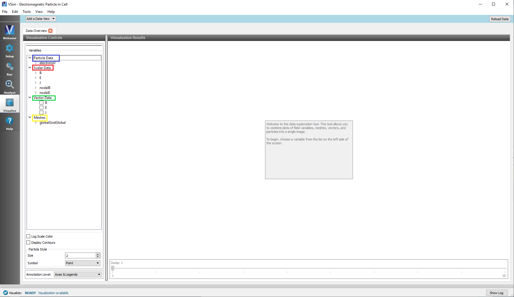
Fig. 104 Particle, Scalar, Mesh Data Variables
Geometries
Types of Geometries include:
- poly
- poly_surface
See Fig. 105.
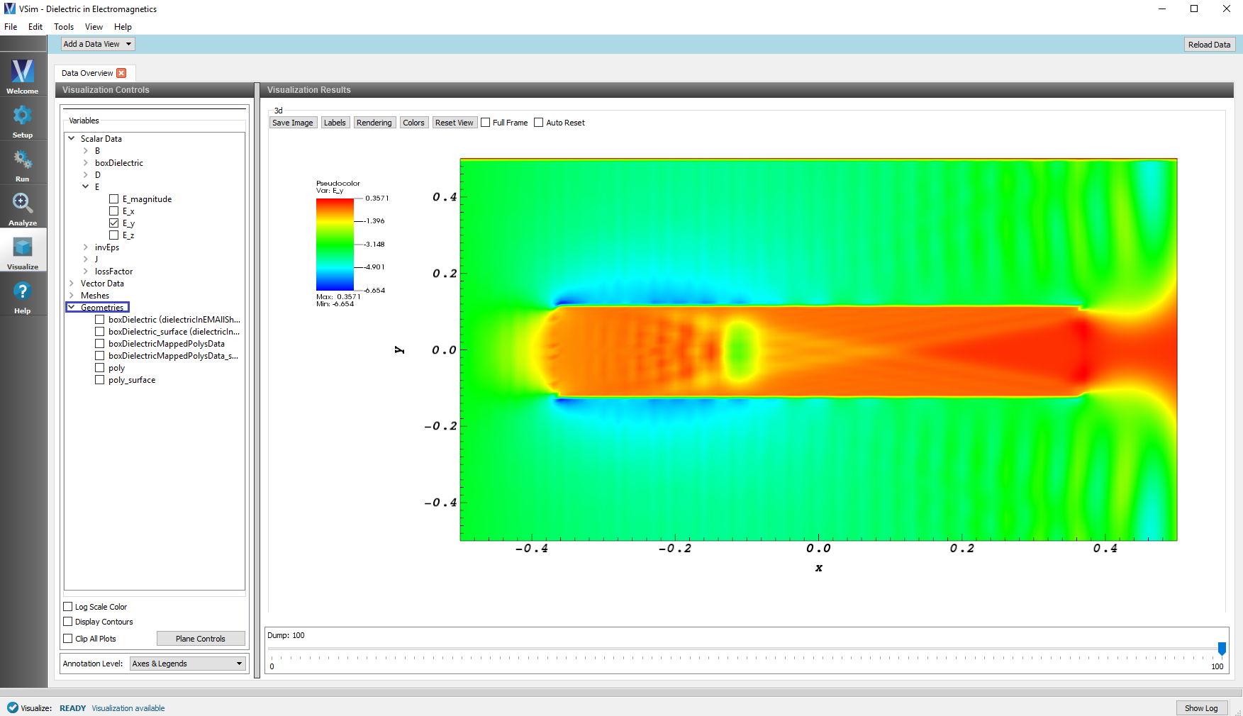
Fig. 105 Geometry Data Variables
Log Scale Color
If the appropriate field is selected, the Log Scale Color checkbox will be available to enable and disable display of log scale color.
Checking this box will put the color on a log scale. This is useful to see details in a field. See Fig. 106.
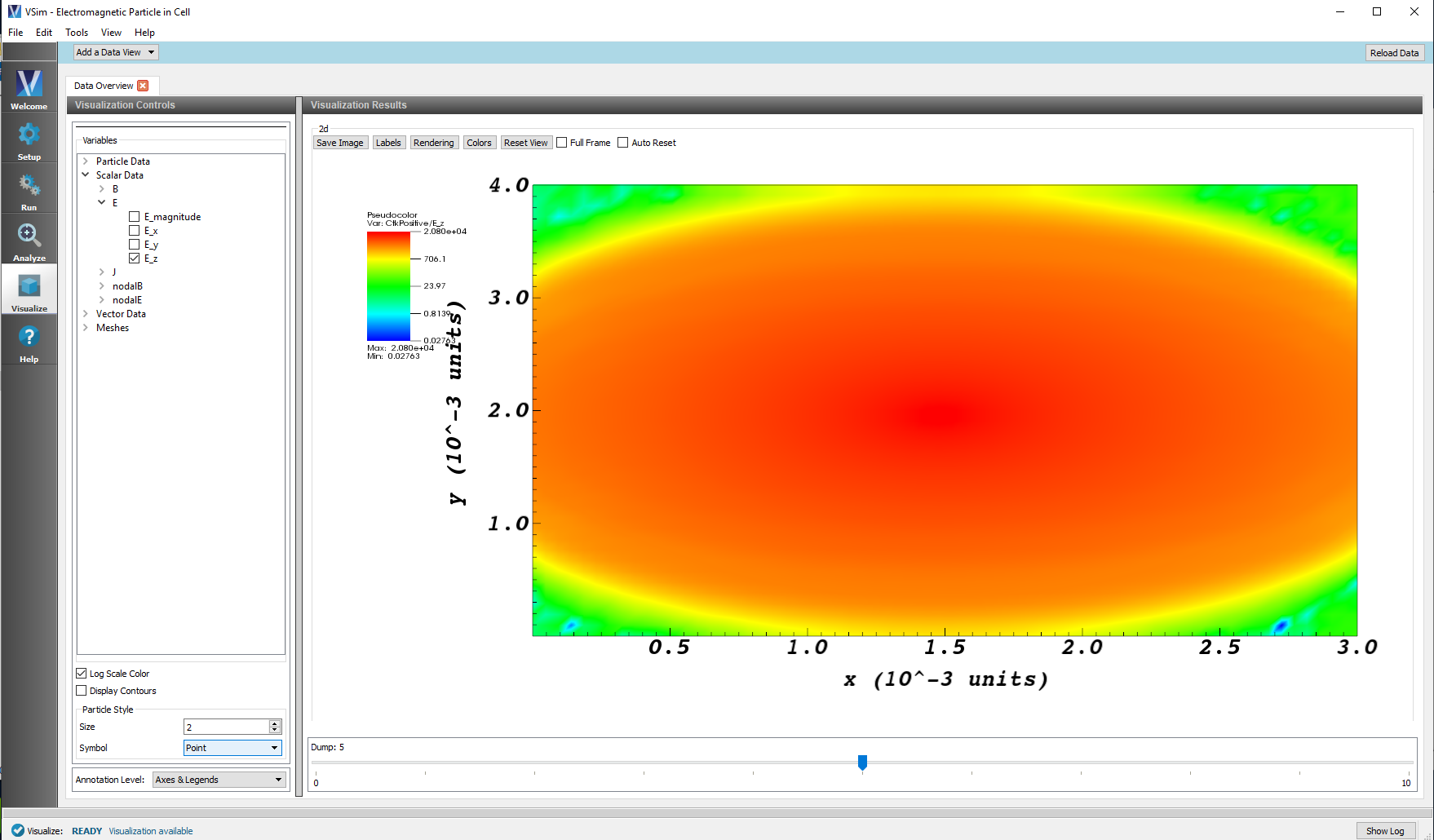
Fig. 106 Log Scale Color Checkbox
Display Contours
The default value in the Contours field is 5. If you select the Display Contours check box and have an appropriate data set selected, the number of contours can be changed to any positive number. See Fig. 107.
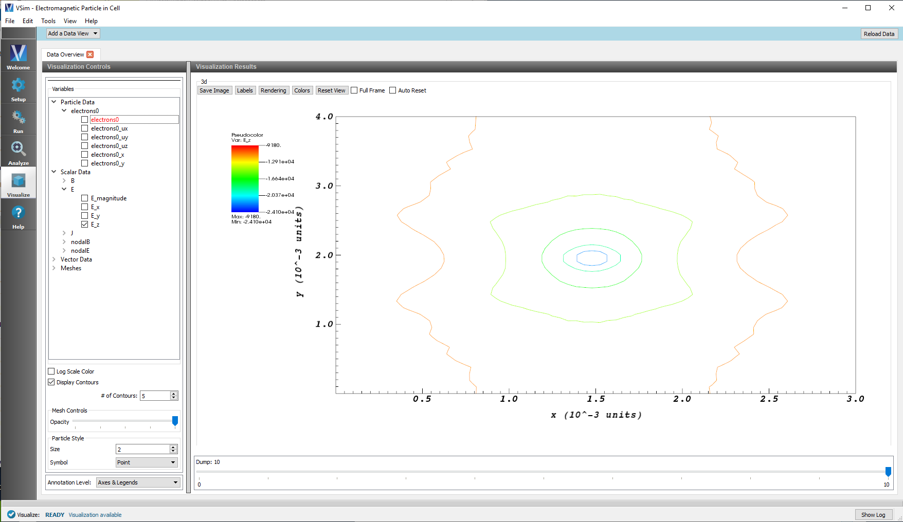
Fig. 107 Contours
Clip All Plots Checkbox
If the appropriate data is selected, the Clip All Plots checkbox will be available to enable and disable plot clipping.
When Clip All Plots is enabled, the Plane Controls can be used to select an axis intercept or normal vector for the clipping. See Fig. 108.
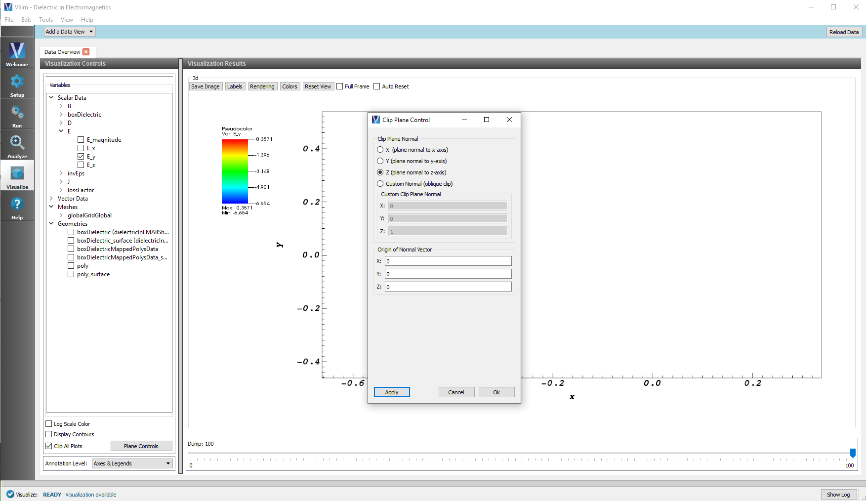
Fig. 108 Clip All Plots Checkbox
Particle Style
The Particle Style section of the Visualization Controls panel enables you to control the appearance of particles in the visualization.
The Size field contains the size of each particle symbol.
The Symbol pulldown menu contains choices for the following shapes:
- Point (default)
- Box
- Axis
- Icosahedron
- Octahedron
- Tetrahedron
- Sphere Geometry
- Sphere
See Fig. 109.
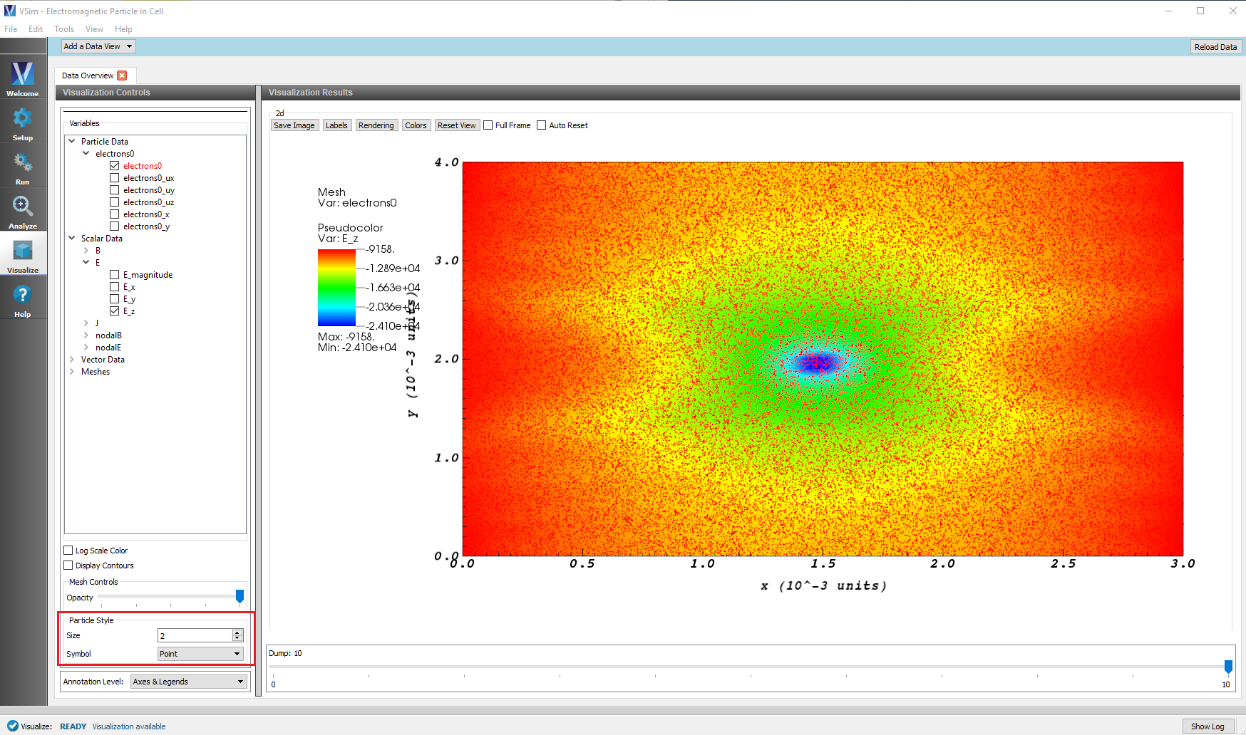
Fig. 109 Particle Style
Field Analysis
The Field Analysis data view will allow further analyzing of a particular field. From the Add Data View drop-down menu in the upper left corner of the pane, select Field Analysis . The Visualization Controls pane allows for selection of the field and selecting the line out location. The Visualization Results pane contains a 2d view of the chosen field, and a lineout at the selected location.
Field
The Field drop-down menu will allow you to choose which field from your simulation to do further analysis on. See Fig. 110.
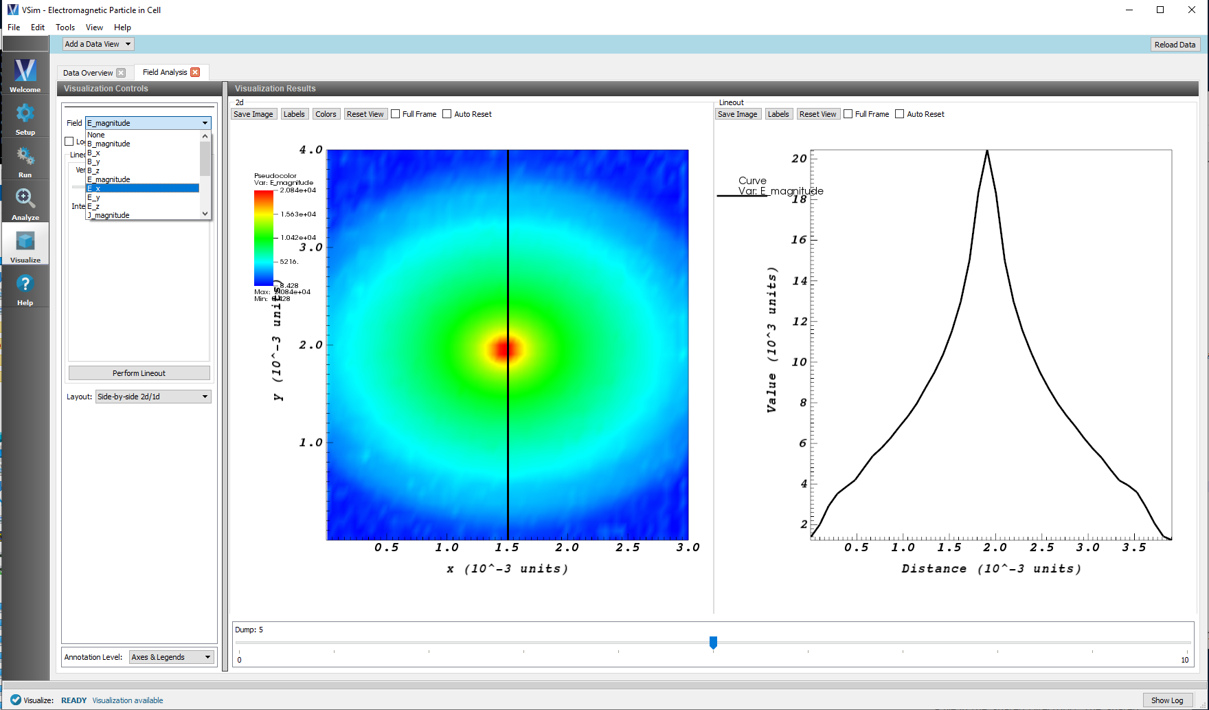
Fig. 110 Field drop down
Slice Settings
Slice settings will appear when a 3D field is viewed. The slice settings allow you to set the position of a slice of the 3D field to create a 2D plot. The Plane Controls botton allows for further control, including creating a slice at an angle. See Fig. 111.
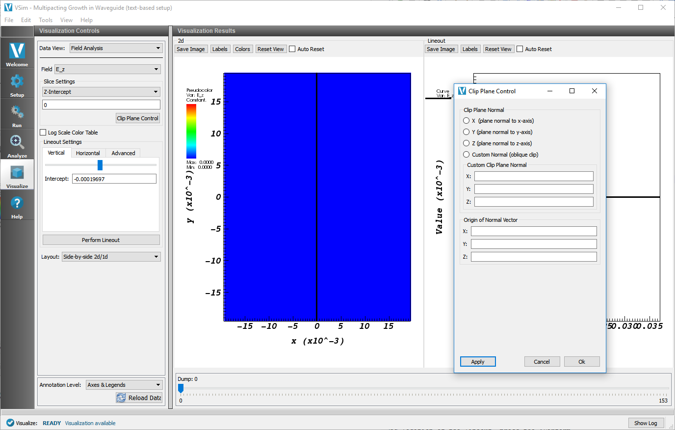
Fig. 111 Slice settings and plane controls for a 3D plot
Log Scale Color Table
Checking this box will put the color on a log scale. This is useful to see details in a field. See Fig. 112.

Fig. 112 Log Scale Color Table Checkbox
Lineout Settings
The position of the lineout can be changed using the Lineout Settings. The lineout can easily be set to vertical or horizontal at a specified intercept location, or the Advanced tab can be used to set a line in any arbitrary direction or length.
After setting the desired location of the lineout, press the Perform Lineout button to replot the lineout. See Fig. 113.
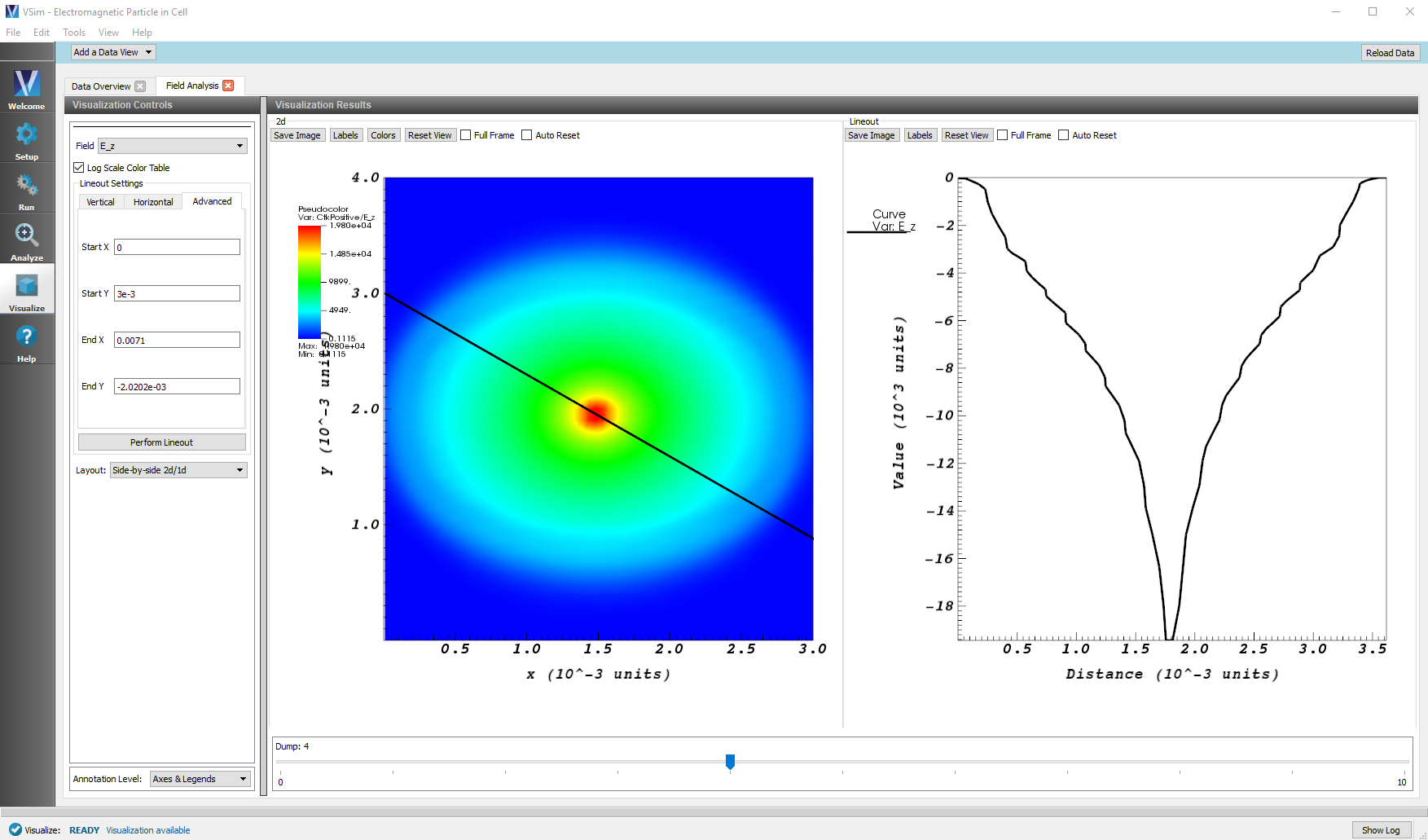
Fig. 113 The lineout settings controls
Layout
The layout of the Visualization Results pane can be changed from the default of Side-by-side 2d/1d. Options include:
- Side-by-side 2d/1d
- Stacked 2d/1d
- 2d Only
- 1d Only
See Fig. 114.
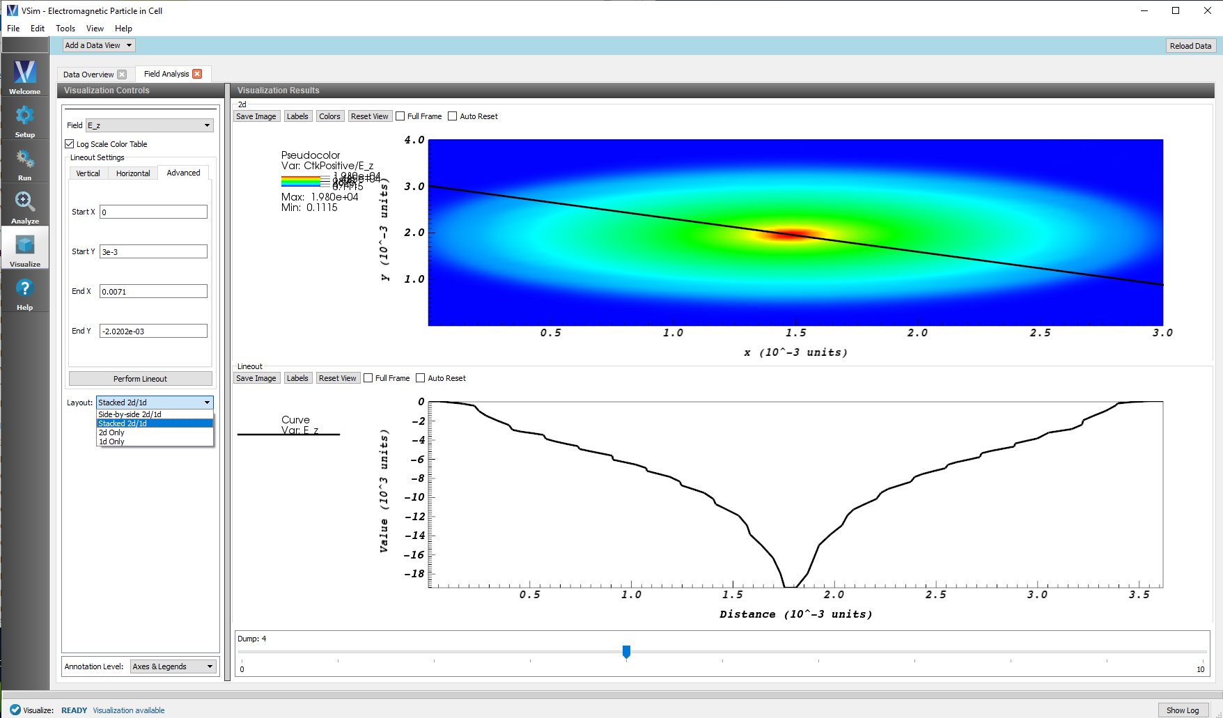
Fig. 114 The layout dropdown options
History
The History data view allows for plotting of any 1D array histories that were included in your input file prior to running your simulation. You can select this from the Add Data View drop-down menu at the top left-hand corner of the pane.
Up to 4 histories can be viewed at one time.
Location
The location drop-down allows you to plot multiple histories on top of each other. By setting the location of graph 1 and graph 2 to Window 1, both plots will appear in the same window.
Color
The color of the line can be modified using the Color drop down. Choices include red, blue, green, and black.
Style
The style of the line can be modified using the Style drop down. Choices include solid, dash, dot, dotdash, and points.
Fourier Amplitude (dB)
Selecting the Fourier Amplitude checkbox will take a Fast Fourier Transform of the data.
Log Scale
Selecting the Log Scale checkbox will put the y-axis on a log scale.
Zoom
Setting the Zoom radial selection will switch the mouse click feature to zoom. Start by clicking the mouse inside the plot window and then dragging to create a rectangle. Finish by un-clicking the mouse button. The plot will be zoomed to the data contained inside the rectangle.
Navigate
Setting the Navigate radial selection will switch the mouse click feature to navigate. Click the mouse inside the plot window and drag to move the plot. See Fig. 115.
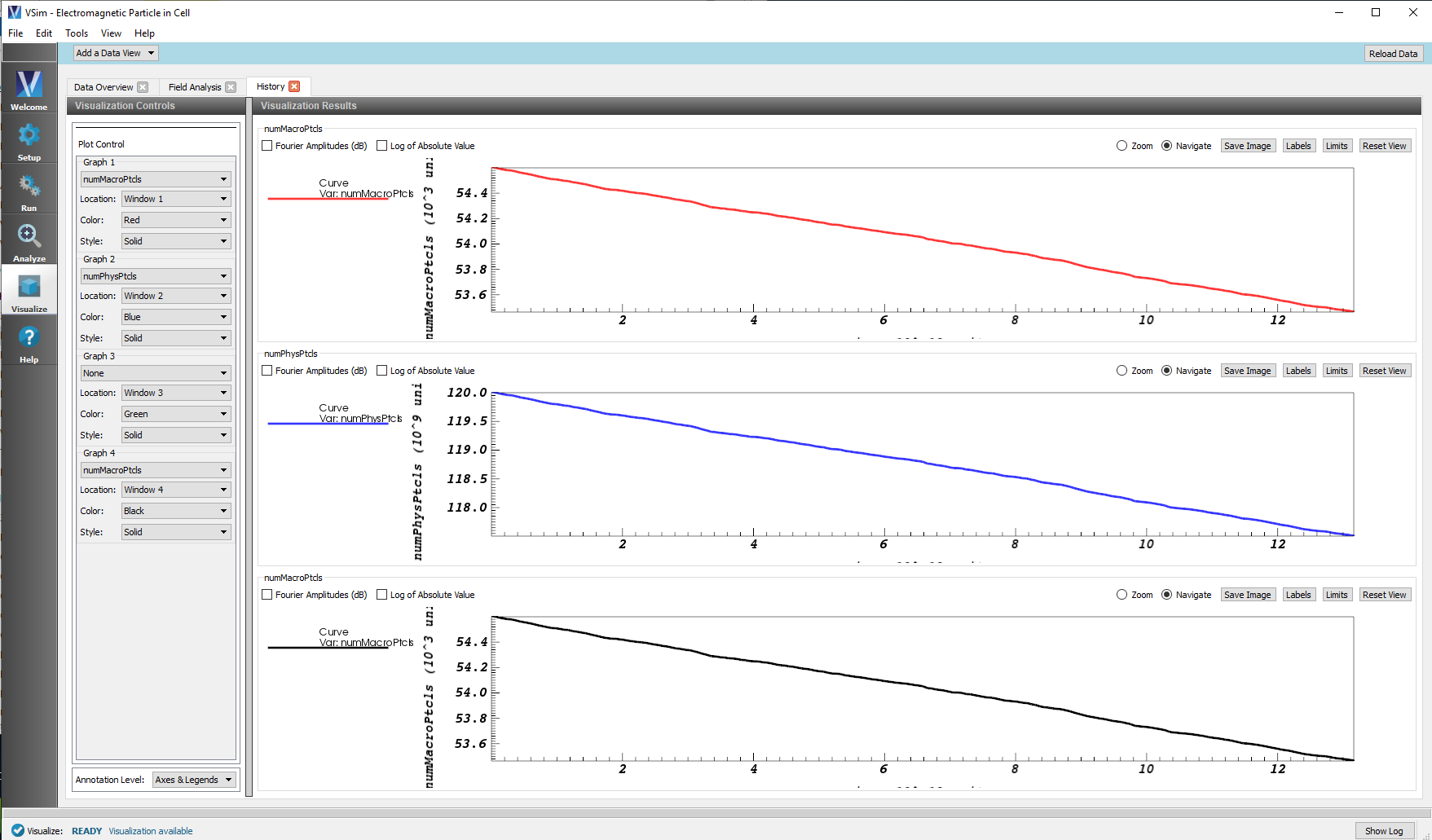
Fig. 115 The History View
Phase Space
The Phase Space data view allows for plotting of any particles (species) in your simulation. You can select this from the Add Data View drop-down menu at the top left-hand corner of the pane.
Base Variable
The Base Variable can be used to switch between any of the particle species in your simulation.
X-axis
The variable to be plotted on the x-axis.
Y-axis
The variable to be plotted on the y-axis.
Z-axis
The variable to be plotted on the z-axis.
Color
The particles can be plotted in either a solid color such as red, green, or blue, or they can be plotted using another variable as their color. An example is to plot the velocity as the color on an x, y, z spatial plot.
Point Size (pixels)
The size of each particle symbol.
Symbol
The Symbol pulldown menu contains choices for the following shapes:
- Point (default)
- Box
- Axis
- Icosahedron
- Octahedron
- Tetrahedron
- Sphere Geometry
- Sphere
Enable Second (Third) Plot
Up to 3 particle species can be plotted at one time in the Phase Space window. To enable another plot, check the box.
Reset View on Draw
When changes are made to the variables to each plot, you must click the Draw button. Check the Reset View on Draw button if you would like the view reset each time the draw button is clicked.
Draw
When changes are made to the variables to each plot, you must click the Draw button to redraw the plot.
See Fig. 116.
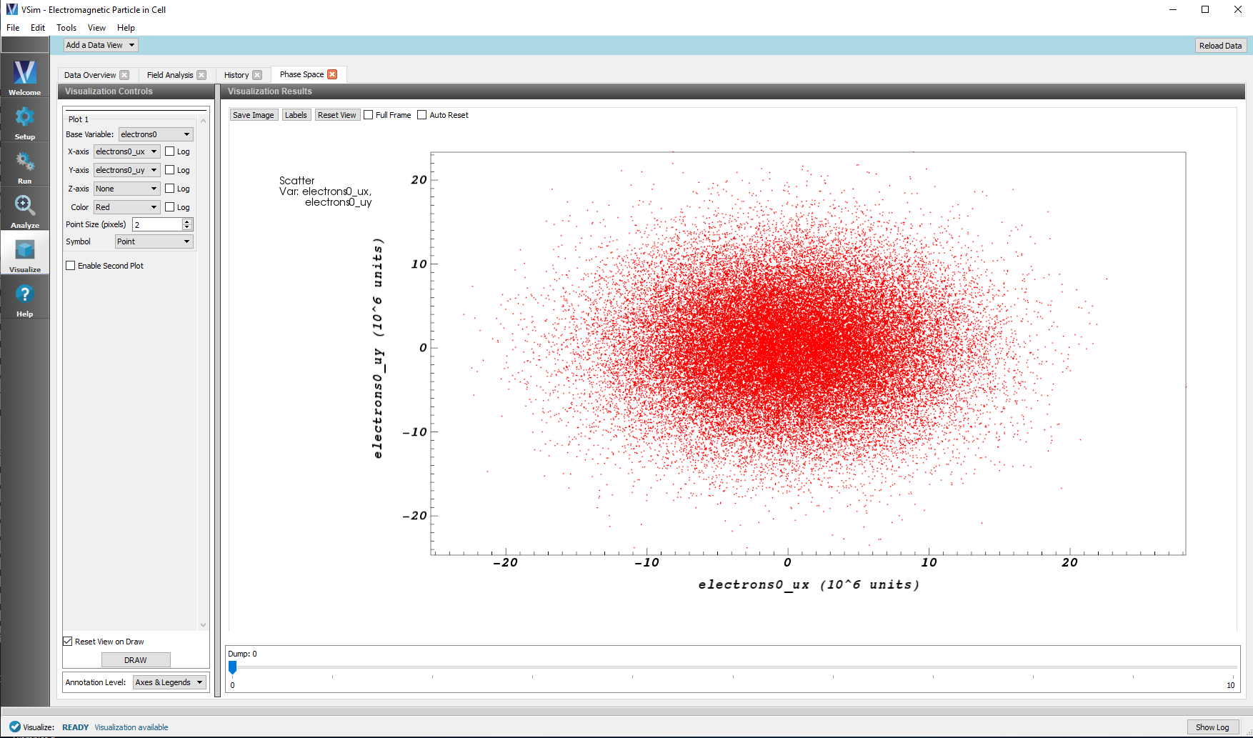
Fig. 116 The Phase Space View
Binning
The Binning data view allows for “binning” the particles (species) in your simulation and creating histogram-style plots. You can select this from the Add Data View drop-down menu at the top left-hand corner of the pane.
Base Variable
The Base Variable can be used to switch between any of the particle species in your simulation.
Variable
The Variable to be binned.
Bins
The number of Bins. The variable will be divided into the number of bins chosen.
Reduction Operator
The Operator is the method used for binning.
Reduction Variable
If the Variable is active (depending on the operator), the variable what the operator acts on.
Draw
When changes are made to the variables, you must click the Draw button to redraw the plot.
Slicing
Slice settings will appear when a third dimension is added. The slice settings allow you to set the position of the slice of the 3D field to create the 2D plot. The Plane Controls button allows for further control, including creating a slice at an angle. See Fig. 117.
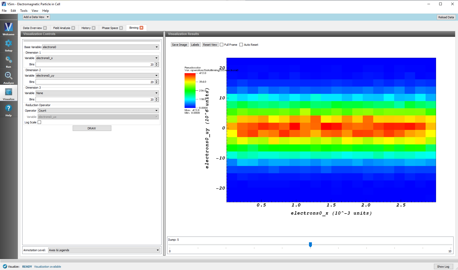
Fig. 117 The Binning View