Satellite Surface Charging (satelliteSurfaceCharge.sdf)

Keywords:

electrostatics, surface charges, Poisson solver

Problem description

Satellites and other spacecraft operating in the space environment often suffer arcing and breakdown problems due to surface charging. Charged particles buildup on the spacecraft surfaces (such as solar panel arrays and other components) leading to localized arcing/breakdown discharges that can critically fail a component or the entire unit. This problem is made worse as the demand for high power space missions in both satellite and deep-space applications rises. These high-power spacecraft are outfitted with high-voltage solar panels. These panels minimize the overall payload requirements and offer other advantages over more massive, low-voltage arrays. However, they are also more vulnerable to surface charge related arcing. It therefore becomes important to predict the surface charge buildup on spacecraft bodies operating in different space environments, where the ion sources may be natural solar wind or human-made space plasma resulting from electric thruster plasma plumes.

This example demonstrates a satellite body operating in the solar wind environment where the space plasma consists of ions and electrons. The simulation box is set up with dimensions of 15 m x 30 m x 15 m. The satellite system is placed in the middle of the domain. It has a 3 m radius x 5 m long cylindrical central unit connected to solar panels at either end. Each solar panel has a total span length of 6 m and a width of 4 m. The satellite central unit has a 5-volt equipotential circular body with radius of 2 m and length of 3 m. The satellite system is treated as a conductor floating in free space which acquires the plasma potential. The system domain boundaries are assumed to have zero perpendicular electric field, i.e. Neumann boundary conditions. The solar wind plasma is introduced in the simulation domain from the positive x direction. The solar wind density is set to \(1 \times 10^{7} \textrm{m}^{-3}\) with a temperature of 10 eV. The number of particles per cell introduced at each time step is 5. The number of physical particles per macro particle is automatically computed by the computational engine (Vorpal). Both electrons and ions are introduced from the source based on the solar wind density and temperature. The electrons and ions and emitted from the XMIN boundary using a particle emitter called a “slab settable flux”. With this emitter, there are many options for specifying the emission quantity such as “emission current density”, “emission flux” and “emission current”. We have chosen to specify the emission current density. For a cold (0 temperature) plasma, the emission current density is \(n0 \times q \times v_d\), where n0 is the number density, q is the charge of the emitted species and \(v_d\) is the drift velocity. For a warm plasma, \(v_d\) must be found as the first moment of the distribution function, which is a drifting Maxwellian. Since the electron thermal velocity is much greater than the ion thermal velocity, this means that the electron current density is also greater than the ion current density. To state this another way, to maintain plasma uniformity within finite bounds, the electron source rate is somewhat larger than the ion source rate because electrons are lighter and leave the system more quickly than do ions. At the same time, the positive ions are imbued with a lighter mass to speed up the simulation. All simulation boundaries are set up to absorb particles. The charges collected in the satellite system are counted by emitting a heavy electron or heavy ion at the point where an electron or ion was absorbed. The heavy electron/ion is not a physical concept, it is a computational trick whereby any charged particle striking the satellite gets converted to a new species, one with equivalent charge but with a much larger mass (1 kg in this case) and suppressed energy (suppressed by a factor of 10 billion). In this way, the heavy particles do not propagate from their point of origin, effectively sticking to the satellite surface. The collected electron and ion currents on the satellite surfaces are output as histories.

This simulation can be performed with a VSimPD license.

Opening the Simulation

The satellite surface charging example is accessed from within VSimComposer by the following actions:

• Select the New → From Example… menu item in the File menu.

• In the resulting Examples window expand the VSim for Plasma Discharges option.

• Expand the Spacecraft option.

• Select “Satellite Surface Charging” and press the Choose button.

• In the resulting dialog, create a New Folder if desired, and press the Save button to create a copy of this example.

All of the properties and values that create the simulation are now available in the Setup Window as shown in Fig. 604. You can expand the tree elements and navigate through the various properties, making any changes you desire. Please note that many options are available by double clicking on an option and also right clicking on an option. The right pane shows a 3D view of the geometry as well as the grid. To show or hide the grid, expand the “Grid” element and select or deselect the box next to Grid. You can also show or hide the different geometries by expanding the “Geometries” and “CSG” elements. Under “CSG”, you will see all the geometries which are created using VSim’s primitive geometry creation capabilities. Selecting a box next to a geometry shows that geometry in the 3D view.

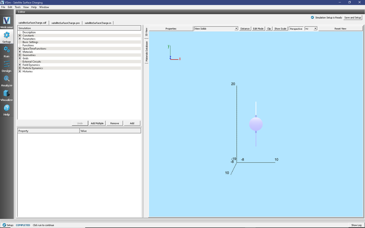
Fig. 604 Setup Window for the Satellite Surface Charging example.

Input File Features

The input file allows a choice of space environment parameters (number density, plasma temperature, drift speed), satellite body voltage, simulation domain size, and resolution (number of cells in each direction). Note, however, that “ION_CURRENT_DENSITY” and “ELECTRON_CURRENT_DENSITY” (which are two parameters that can be found by expanding the “Parameters” option) are computed outside of VSim. These are found by computing the first moment of the drifting Maxwellian which is the kinetic drift velocity that takes in to account the thermal spread of each species. Therefore, if you change the number density, plasma temperature and/or drift speed, “ION_CURRENT_DENSITY” and “ELECTRON_CURRENT_DENSITY” will need to be recomputed. The current density for species \(s\) can be found with the following formula: \(n0 \times q_s \times \int_{-\infty}^{0} vf(v) \mathrm{d}v\) , where \(f(v)\) is the kinetic distribution function which is represented as a drifting Maxwellian in this example. Note that the integral extends from \(-\infty\) to 0 since this is the range of particles that get injected from the XMIN boundary.

The self-consistent electric field is solved from Poisson’s equation by the electrostatic solver. The far-field space boundaries are handled with Neumann boundary conditions. The satellite inner body is set up with an equipotential boundary. The surface charges collected on the satellite system make the satellite body float at a slightly lower voltage than the space plasma.

The plasma is represented by macro-particles which are moved according to the Boris pusher.

Running the simulation

After performing the above actions, continue as follows:

• Proceed to the run window by pressing the Run button in the left column of buttons.

• To run the file, click on the Run button in the upper left corner of the right panel. You will see the output of the run in the right pane. The run has completed when you see the output, “Engine completed successfully.” This is shown in Fig. 605.

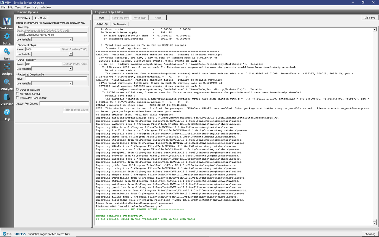
Fig. 605 The Run Window at the end of execution.

Analyzing the Results

If the electron density is desired, then proceed as follows:

• In the leftmost panel, click the Analyze button and then select computePtclNumDensity.py from the list of analyzers, then click Open at the top of the Analysis Controls pane.

• Enter the following parameters in the appropriate fields:

  • simulationName = satelliteSurfaceCharge

  • speciesName = solarWindElectrons

  • avgNxN = 1

  • iterateAvg = 1

• Click the Analyze button in the upper right corner of the window.

See Fig. 606.

The resulting data can be visualized as solarWindElectronsDensity under the Scalar Data menu in the Visualize Tab. The density of solarWindIons can be calculated in the same way by substituting that species name in place of solarWindElectrons.

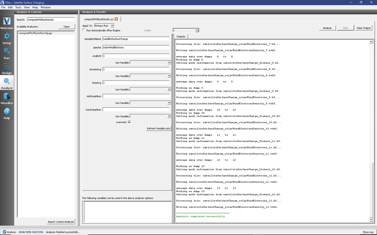
Fig. 606 The Run Window at the end of execution.

Visualizing the results

After performing the above actions, proceed to the Visualize Window by pressing the Visualize button in the left column of buttons.

To visualize the satellite geometry with electrons proceed as follows:

• Open a Data Overview tab.

• Expand Particle Data.

• Expand heavySolarWindElectrons.

• Select “heavySolarWindElectrons” in red.

• Expand solarWindElectrons.

• Select “solarWindElectrons” in green.

• Expand Geometries.

• Select “poly_surface (satelliteWithRodsUnionsatelliteBothCells)”.

• Move the Dump slider to dump 7.

The resulting plot is shown in Fig. 607. In order to view the data as shown in Fig. 607, you need to take a slice in the z=0 plane. To do this, click on “Plane Controls”, then select Z(plane normal to z-axis) to be the plane normal. Finally, set the Origin of Normal Vector to be 0.0 and click OK. You need to follow these steps for all the data shown. Therefore, do this after selecting “heavySolarWindElectrons” and “solarWindElectrons”.

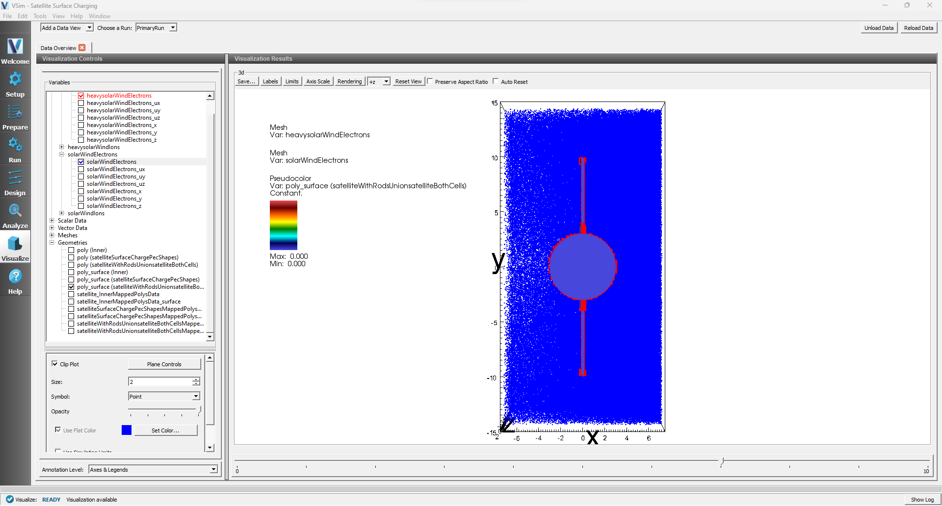
Fig. 607 Visualization plot of satellite system with solar wind electrons in green and the electrons that stick to the satellite surface in red.

Here are some things to try:

• Under Data Overview you can access plots of the electric field, charge density (ChargeDensity), and electric potential (Phi). To view these data sets, expand Scalar Data option. After selecting any field quantity, to view a slice in plane, click on “Plane Controls” as discussed above

• To view the phase space distribution for the electrons and ions, click on the Add a Data View drop down menu and select Phase Space. Click the Draw button to generate a plot.

• Also from the Data View menu select History to observe the satellite currents and the time history results for the number of macro-particles broken down by species.

To generate Fig. 608, that shows the satellite system with the inner equipotential cylindrical body, proceed as follows:

• In the Data View pane on the left side select “Data Overview” from the drop-down menu.

• Expand Geometries

• Select “poly (satelliteWithRodsUnionsatelliteBothCells)”

• Select “poly_surface (Inner)”.

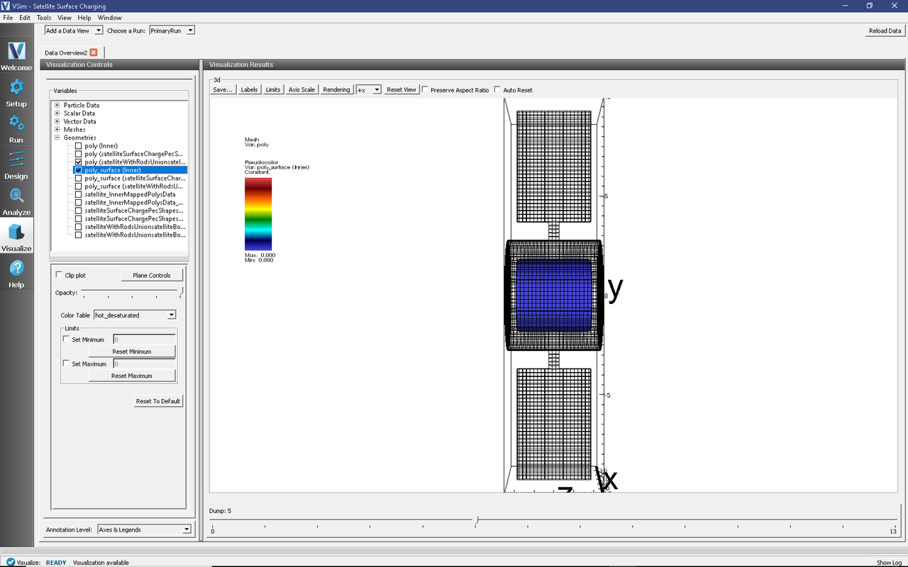
Fig. 608 Visualization of the inner body inside the satellite system.

The spatial distribution of the positive ions (solarWindIons species) surrounding the satellite system is shown in Fig. 609 which is obtained after running the simulation for 400 time steps. Solar wind plasma enters into the simulation system from the minimum x boundary. If the plane is still clipped from prior plots, uncheck the “Clip plot” box next to the “Plane controls” button. Furthermore, play around with the different colors and opacity options until a plot with the desired look is achieved. There is also an “Annotation levels” option at the bottom of Composer. We have selected “No annotations” so that just the satellite is showing.

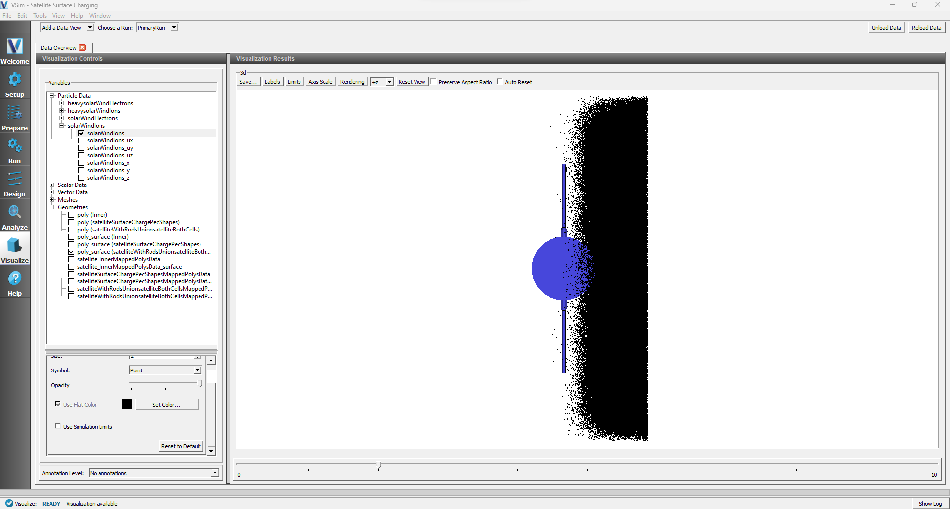
Fig. 609 Visualization of the satellite system with solar ions.

The charge density on the satellite system is shown in Fig. 610 after running for 2,000 time steps. To view the charge density in the simulation domain, click on “Add a Data View” and choose “Field Analysis”. Then click on region next to “Field” and choose ChargeDensity. The default view will show a 3D, 2D and 1D view (i.e. 3 windows are shown by default). You can choose different slices in the 3D view just as you could in the Data Overview tab. To view the data as shown in Fig. 610, click in the region next to “Layout” and choose “Side-by-side 2d/1d”. Now we want to make the color scale symmetric with respect to 0. So click on “Colors above the 2D color contour plot. Then check the boxes “Fix Minimum” and “Fix Maximum” and choose the color scale to lie between -2e-11 and 2e-11 (units are in \(\mathrm{C}/\mathrm{m}^3\)). Next, for the lineout setting, click on “Horizontal” and drag the bar to change the location of the lineout. This allows you to quantify the data better. We see in this plot a large negative build-up on the side the solar wind enters from and a smaller build-up on the opposite side of the satellite. We have circled some of the key features in Composer that allow you to customize your plot.

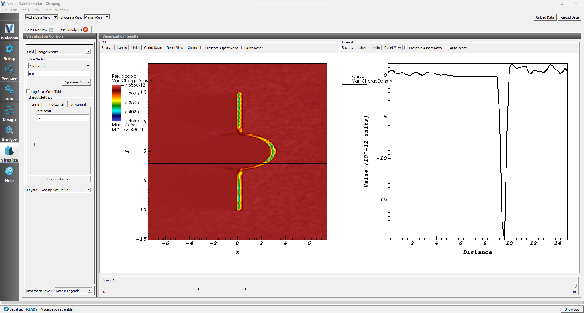
Fig. 610 Visualization of the charge density on the satellite system.

To view the electrostatic potential, check the box next to “Phi” under the Scalar Data in the Data Overview pane. The electrostatic potential of the satellite system simulated is shown in Fig. 611 after running for 2,000 time steps. The electrostatic potential is plotted in the X-Y-Z domain with clipping in the Z=0 plane. The bulk of the plasma potential in the space region is close to -1 V (red region). The negative surface charge built-up on the solar panels lowers the surface potential about 5 V below the bulk space plasma.

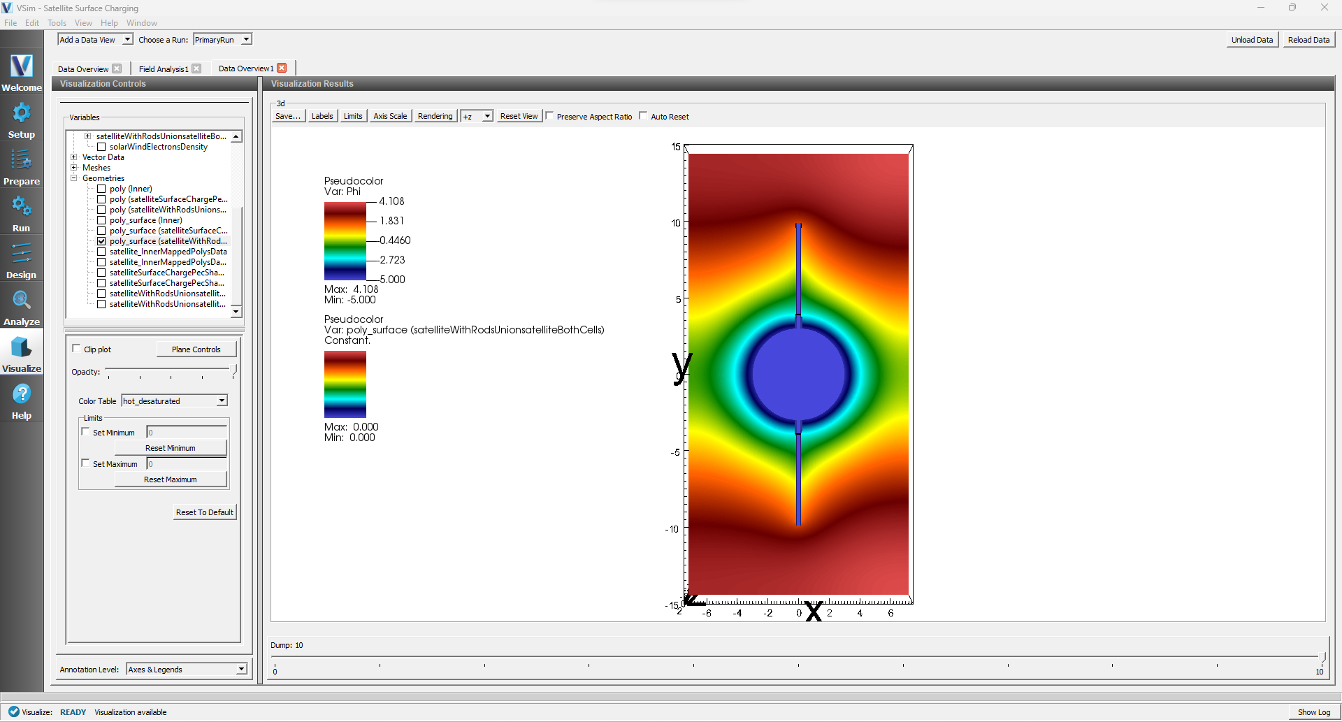
Fig. 611 Visualization of the electric potential surrounding the satellite system.

Further Experiments

The geometry and background space plasma parameters of this input file can be modified to test satellite inner body voltages and satellite surface charge collection in a variety of different space environments.