Coupon Array Charging (couponArrayCharging.sdf)

Keywords:

solar wind, electrostatics, surface charging

Problem description

In orbit, insulating outer surfaces of satellites will develop a surface charge due to the impinging solar wind. If enough surface charge accumulates electric breakdown can occur across or through the satellite and damage the craft.

This simulation models the accumulation of solar wind particles on an array of solar cells (coupons). The array includes 6 coupons, a kapton backing, and 6 metal busbars. Using post-simulation analysis, the component of the electric field normal to the surface of the satellite is calculated.

With additional data specific a particular spacecraft and materials, this simulation can indicate locations where breakdown is likely to occur.

NOTE: The simulation runs in serial and on 4 cores out of the box in Windows. On Linux, the example runs on up to 12 cores (testing above 12 cores has not been done).

This simulation can be performed with a VSimPD license.

Opening the Simulation

The Electron Drifting example is accessed from within VSimComposer by the following actions:

• Select the New → From Example… menu item in the File menu.

• In the resulting Examples window expand the VSim for Plasma Discharges option.

• Expand the Spacecraft option.

• Select “Coupon Array Charging” and press the Choose button.

• In the resulting dialog, create a New Folder if desired, and press the Save button to create a copy of this example.

The Setup Window as seen after opening the example is shown in Fig. 591.

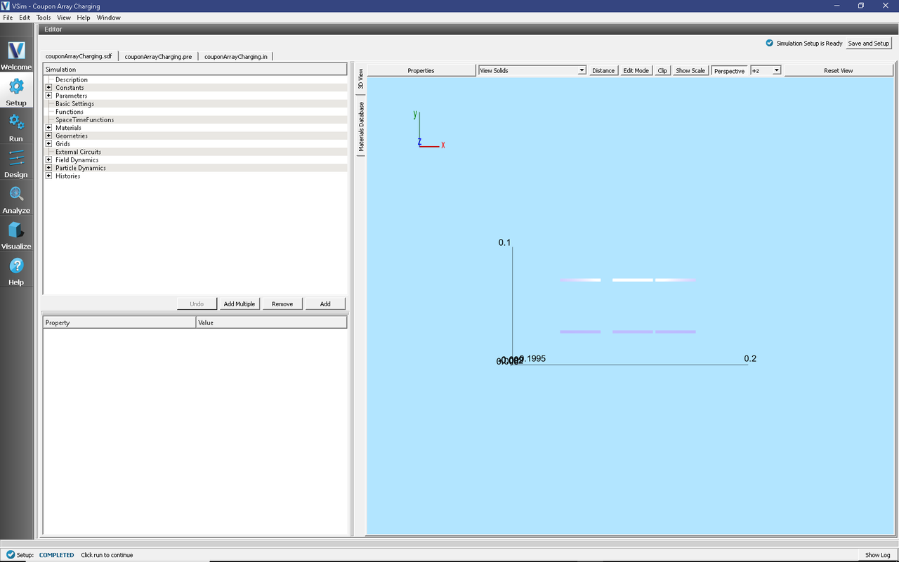
Fig. 591 Setup Window for the Coupon Array Charging example.

Simulation Properties

The geometry for the busbars and coupon array are imported from stl files. Material properties are set on the geometries: perfect electrical conductor (PEC) for the busbars, and absorbium, an insulating particle absorbing material, on the array of cells.

A voltage of 5 volts is set on the busbars. The upper z boundary is set as the \(V = 0\) point, a Neumann boundary condition is set on the lower z boundary of the simulation grid, which enforces that the gradient of the electric field normal to this surface is zero. Periodic boundary conditions (for particles and fields) are set on all other simulation boundaries.

The solar wind is emitted off the upper z boundary of the simulation domain with a number density of 1.e7 particles per meter cubed. The masses of the ions are artificially set to 100x the mass of the electrons. Particle accumulation boundary conditions are set on the insulating surface of the coupons, and a particle absorbing boundary condition is set on the metal busbars.

Histories save the absorbed particle energy deposited onto the satellite surface.

Running the Simulation

After performing the above actions, continue as follows:

• Proceed to the Run Window by pressing the Run button in the left column of buttons.

• To run the file, click on the Run button in the upper left corner of the Logs and Output Files pane. You will see the output of the run in this pane. The run has completed when you see the output, “Engine completed successfully.” This is shown in Fig. 592 below.

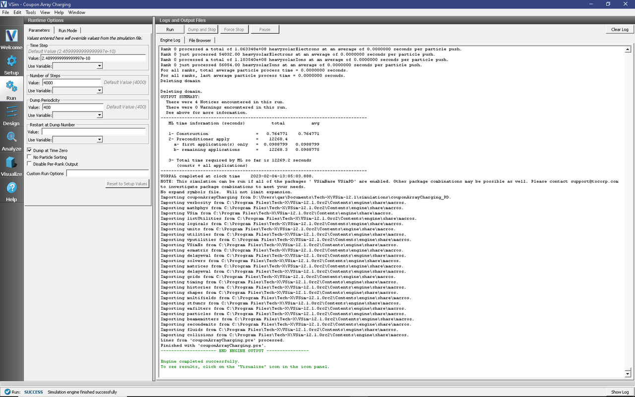
Fig. 592 The Run Window at the end of execution.

Analyzing the Results

The physics engine, vorpal, inside VSim only calculates field values on edges, nodes, or faces of grid cells. The putFieldOnSurfaceMesh.py analyzer can interpolate the values calculated on the grid to the surface of a geometry in the simulation.

To calculate the normal component of the electric field on the surface of the array, proceed to the Analyze Tab. The putFieldOnSurfaceMesh.py analyzer is included by default to this simulation. Click on the text “putFieldOnSurfaceMesh.py (Default)” to highlight it, then click the “Open” button at the bottom of the Analysis Controls pane. Ensure the following is entered into each field:

• simulationName: “couponArrayCharging”

• geometryName: “satelliteSurfaceGeomSolid”

• fieldName: “E”

• beginDump: “1”

• endDump: “9”

• outputFileName: “elecFieldOnSurface”

• Click Analyze in upper right corner of the window. When the analysis is finished, you should see a window similar to Fig. 593.

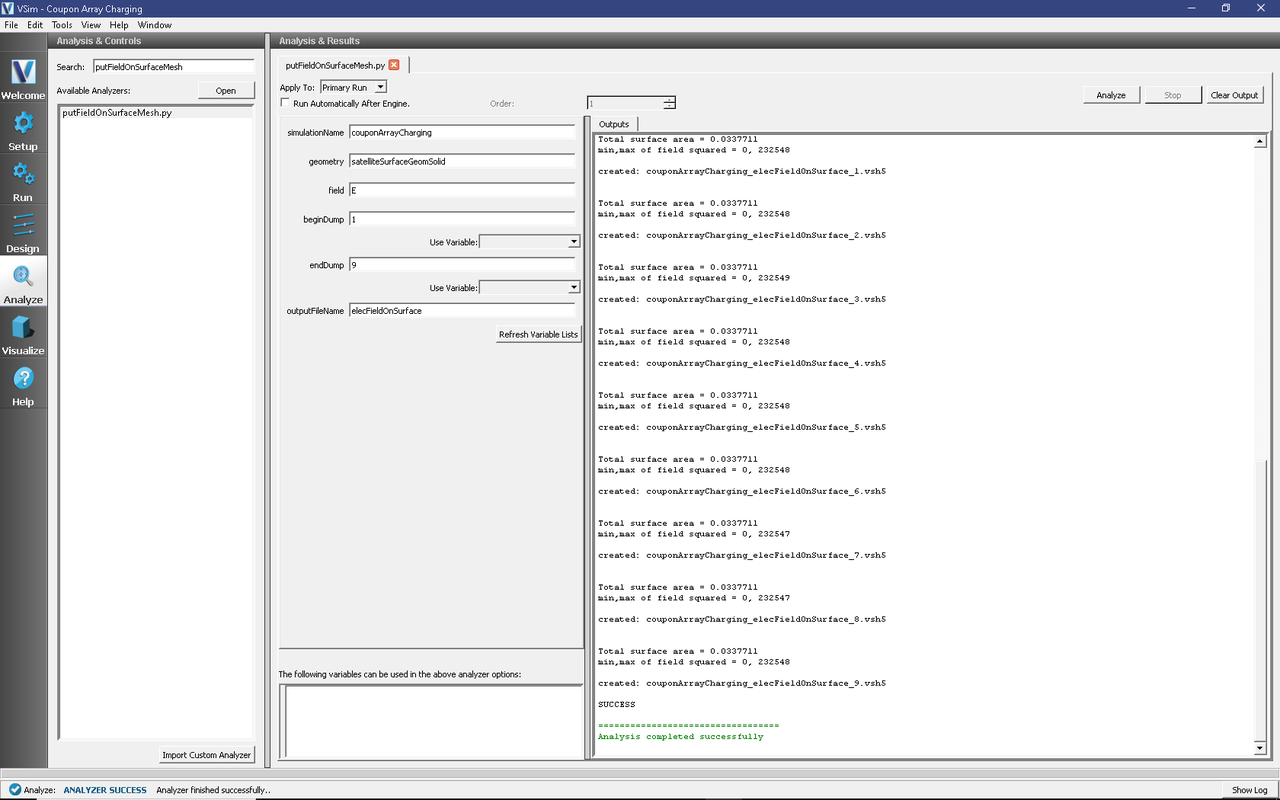
Fig. 593 The Analyze Window at the end of execution.

Visualizing the Results

After run completion, continue as follows:

Proceed to the Visualize Tab by pressing the Visualize button in the left column of buttons. To view the normal component of the electric field on the surface of the array follow the following steps.

• If you have previously switched to the Visualize Tab, you will have to click the Reload Data button at the bottom of the Visualization Controls pane.

• In the upper left corner of the Visualization window, click on “Add a Data View” and select “Data Overview” (note: there may already be a “Data Overview” tab opened. If so, skip this step.)

• In the “Data Overview” tab, expand “Scalar Data” then expand “elecFieldOnSurface” and check the box for “elecFieldOnSurface_magnitude” to plot the component of the electric field normal to the surface of the coupon array. It is also possible to plot the two tangential components of the field, as well as the magnitude.

• To compare to the satellite geometry, expand “Geometries” then select “poly (satelliteSurfaceGeomSolid)”.

• To see the fields more clearly, select “Log Scale Color”

• The resulting visualization is shown in Fig. 594.

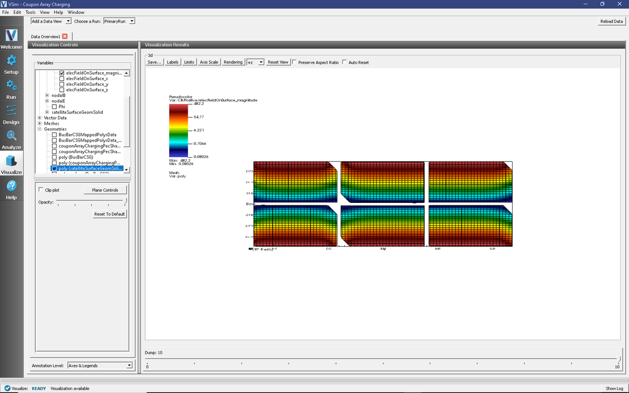
Fig. 594 Visualization of the Electric Field on the Satellite Surface.

We can see the accumulation of electric charge by unselecting “elecFieldOnSurface_magnitude” and viewing “ChargeDensity” instead. To view the charge density on the surface of the geometry, click on “Plane Controls” with your mouse. A new window will pop open. In the new window, make sure that the “Z (plane normal to z-axis)” is checked and that “Origin of Normal Vecor” is such that Z=0. Also make sure that the box next to “Clip Plot” is checked. Note that we are plotting the data on a log color scale. Move the dump slider to view the accumulation of charge over time, as shown in Fig. 595.

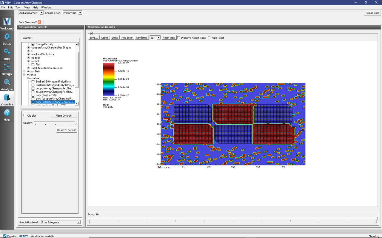
Fig. 595 Visualization of the Charge Density

Further Experiments

Perform the same analysis done above for the electric potential, “Phi,” and charge density, “ChargeDensity,” to create plots of those fields on the surface of the satellite geometry.

Import your own geometry and reset the materials, grid size, and particle absorbers as necessary.

Increase the grid resolution to get finer data on the electric field that develops on the surface of the spacecraft.

Change the number density and speeds of the incident particles to values for orbits at different altitudes.