Spherical Lens (sphericalLens.sdf)
Keywords:
- refraction, focusing, dielectrics
Problem Description
The Spherical Lens is a full wave solution to a simple, thin lens with spherical surfaces. Focusing occurs because light rays farther from the center hit the surface at a more oblique angle, resulting in more bending, according to Snell’s law. The focusing length of a spherical lens is given by \(f = R/(2 - 2/ \epsilon_r^{1/2})\), where \(\epsilon_r\) is the relative permittivity of the material making up the lens.
This simulation can be performed with a VSimEM license.
Opening the Simulation
The Spherical Lens example is accessed from within VSimComposer by the following actions:
Select the New → From Example… menu item in the File menu.
In the resulting Examples window expand the VSim for Electromagnetics option.
Expand the Other EM option.
Select “Spherical Lens” and press the Choose button.
In the resulting dialog, create a New Folder if desired, and press the Save button to create a copy of this example.
All of the properties and values that create the simulation are now available in the setup window as shown in Fig. 327. You can expand the tree elements and navigate through the various properties, making any changes you desire. The right pane shows a 3D view of the geometry, if any, as well as the grid, if actively shown. To show or hide the grid, expand the Grid element and select or deselect the box next to Grid.
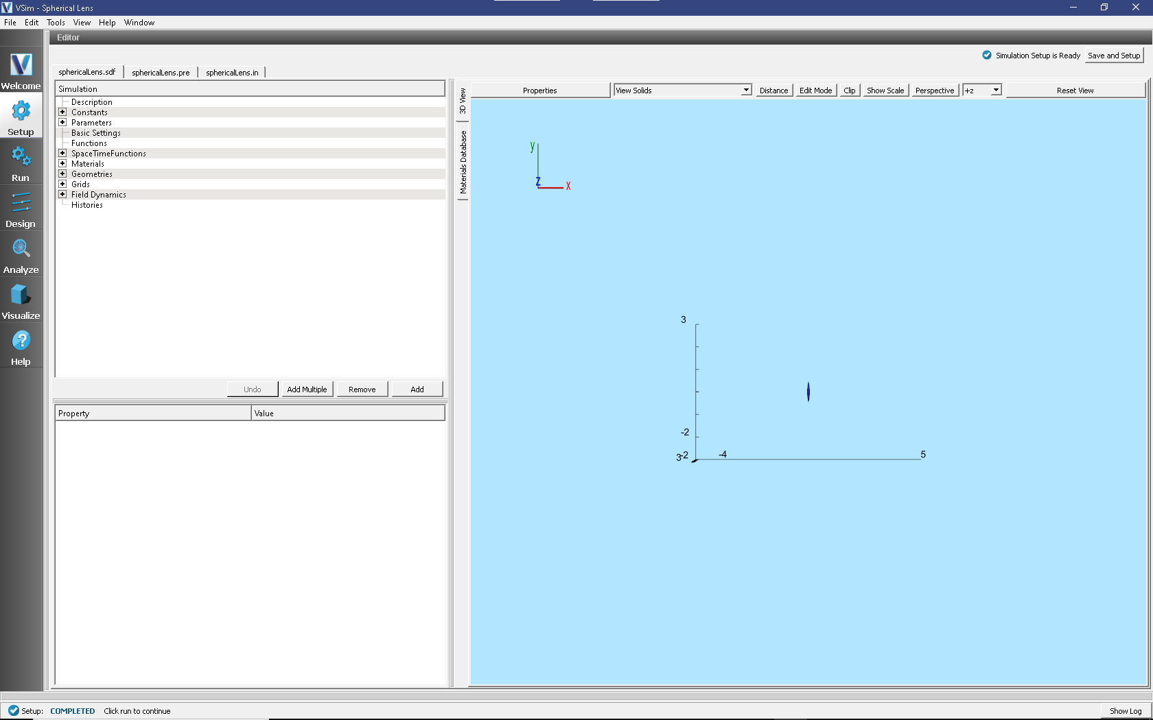
Fig. 327 Setup window for the Spherical Lens example.
Simulation Properties
The spherical lens is constructed in CSG using the intersection of two spheres. You can pull the spheres apart to get a taller lens, and you can change the radius of the spheres to have a lens with more curvature. The grid is set so that it will capture the focus at the right for the initial setup.
Running the Simulation
After performing the above actions, continue as follows:
Proceed to the run window by pressing the Run button in the left column of buttons.
To run the file, click on the Run button in the upper left corner of the right panel. You will see the output of the run in the right pane. The run has completed when you see the output, “Engine completed successfully.” This is shown in Fig. 328.
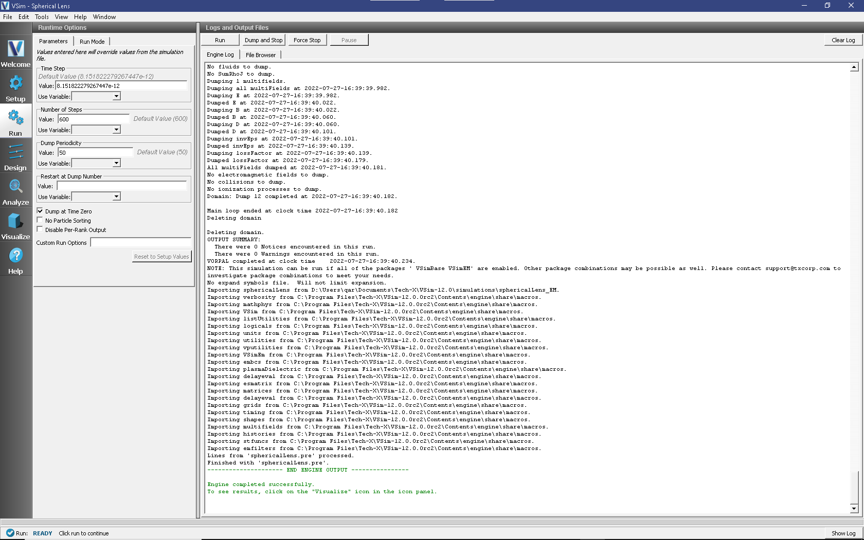
Fig. 328 The Run window at the end of execution.
Visualizing the results
After performing the above actions, continue as follows:
Proceed to the Visualize window by pressing the Visualize button in the left column of buttons.
To see the field focus after the lens as shown in Fig. 329, do the following:
Expand Scalar Data, expand E
Select E_z and check the box Clip Plot
For the limits set the Fix Minimum to -10 and the Fix Maximum to 10.
Expand Geometries
Select poly and check the box Clip Plot
Move the dump slide to the right to see the wave come in, focus after the lens, and then diverge again after approximately x=0.4. One can see interference of the incoming wave with the reflection off the face of the lens. One can also see interference patterns within the lens.
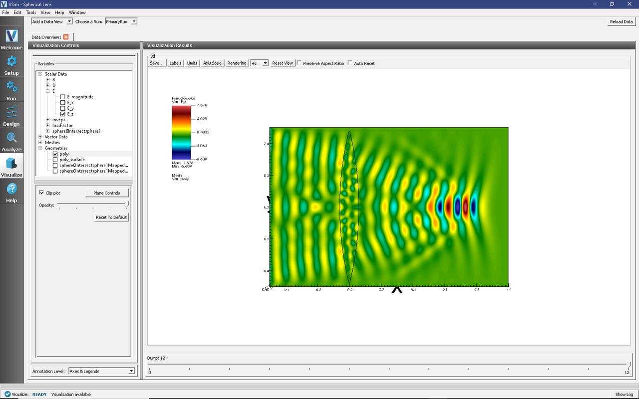
Fig. 329 Visualization of the lens focusing
Further Experiments
Use a material of larger dielectric constant to see more focusing.
Reduce the sphere radii to have more focusing.