Radar Cross Section of a Cylinder (radarCrossSectionT.pre)
Keywords:
-
RCS, far field, radar cross section
Problem description
This simulation launches a plane wave, polarized in the Y-direction at a conducting cylinder in free space. After the plane wave has been launched the Radar Cross section is computed. This problem is a template to solve any Bistatic radar cross section problem.
This simulation can be performed with a VSimEM license.
Opening the Simulation
The radarCrossSectionT example is accessed from within VSimComposer by the following actions:
- Select the New → From Example… menu item in the File menu.
- In the resulting Examples window expand the VSim for Electromagnetics option.
- Expand the Advanced Examples (Text-based setup) option.
- Select “Radar Cross Section” and press the Choose button.
- In the resulting dialog, create a New Folder if desired, and press the Save button to create a copy of this example.
The key parameters of this problem should now be alterable via the text boxes in the left pane of the Setup Window, as shown in the figure Fig. 284.
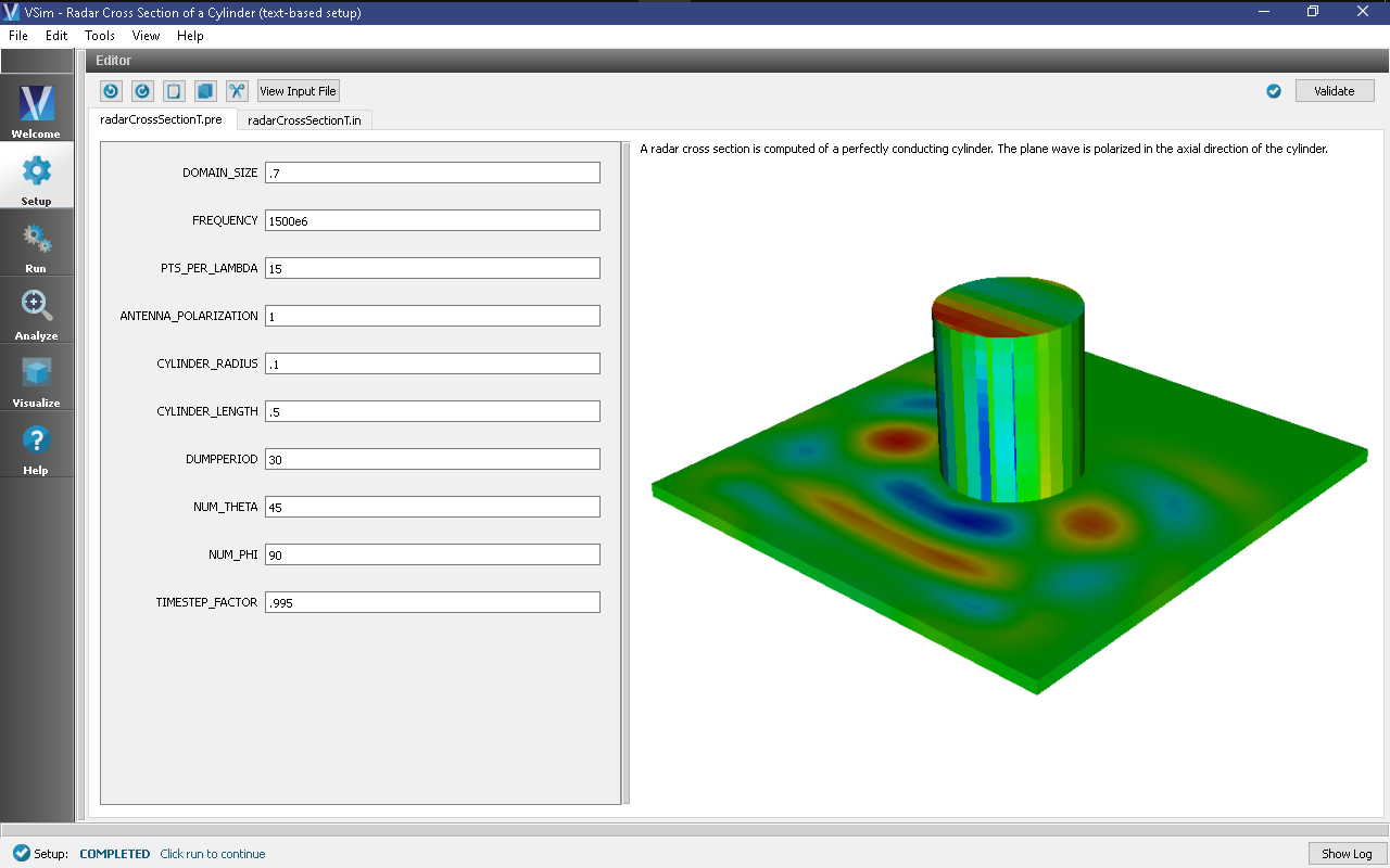
Fig. 284 Setup Window for the Radar Cross Section example.
Input File Features
This file allows the modification of plane wave operating frequency, orientation, simulation domain size and far field resolution. This file has had its accuracy reduced marginally in order to reduce run time. It is generally recommended that between 10 and 20 points per wavelength are used for full accuracy.
Running the Simulation
After performing the above actions, continue as follows:
- Proceed to the Run Window by pressing the Run button in the left column of buttons.
- To run the file, click on the Run button in the upper left corner of the Logs and Output Files pane. You will see the output of the run in that pane. The run has completed when you see the output, “Engine completed successfully.” This is shown in Fig. 285
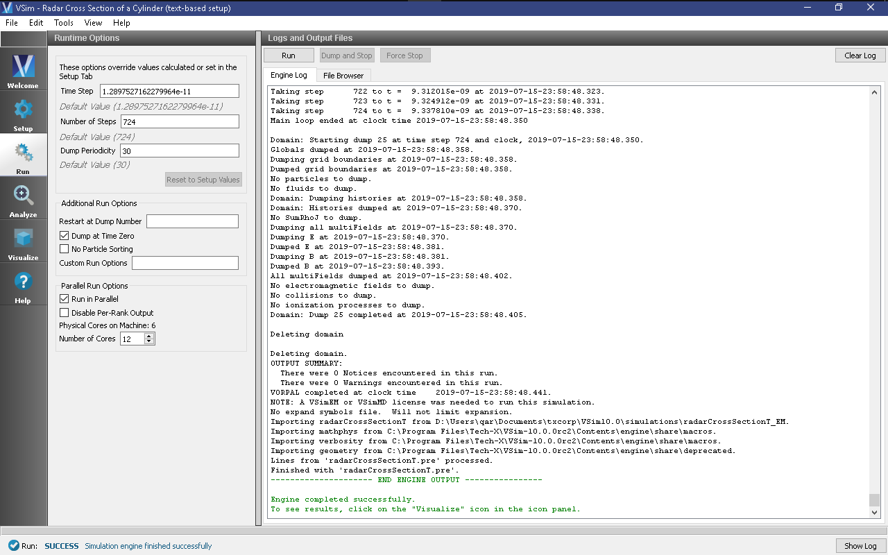
Fig. 285 The Run Window at the end of execution.
Analyzing the Results
To calculate the radar cross section at far field, complete the following steps:
- Proceed to the Analysis window by pressing the Analyze button in the left column of buttons.
- In the list of Available Analyzers, select computeFarFieldFromKirhhoffBox.py (Fig. 286) and press Open.
- Input values for the analyzer parameters. The analyzer may be run
multiple times, allowing the user to
experiment with different values.
- simulationName - radarCrossSectionT (name of the input file)
- fieldLabel - E (name of the electric field)
- farFieldRadius - 10.0 (distance to far field in m, 10.0 is a good value)
- timeStepStride - 20 (number of timesteps between far field calculations; determines how many far fields are output; 20 steps should yield 4 far fields in this case)
- getFourierComponent - 0 (whether to fourier analyze for a particular frequency)
- frequency - the frequency to use in the fourier analysis (not needed here).
- numTheta - 60 (number of theta points in the far field, 18 for a quick calculation, 45 for finer resolution)
- numPhi - 120 (number of phi points in the far field, 36 for a quick calculation, 90 for finer resolution)
- zeroThetaDirection - (0,0,1) (determines orientation of far field coordinate system)
- zeroPhiDirection - (1,0,0) (determines orientation of far field coordinate system
- varyingRadiusMesh - 0 (Set to 1 in order to make far field mesh adapt to magnitude of far field solution: the classic lobe view)
- simpsonIntegration - 0 (Set to 1 for more accurate integration)
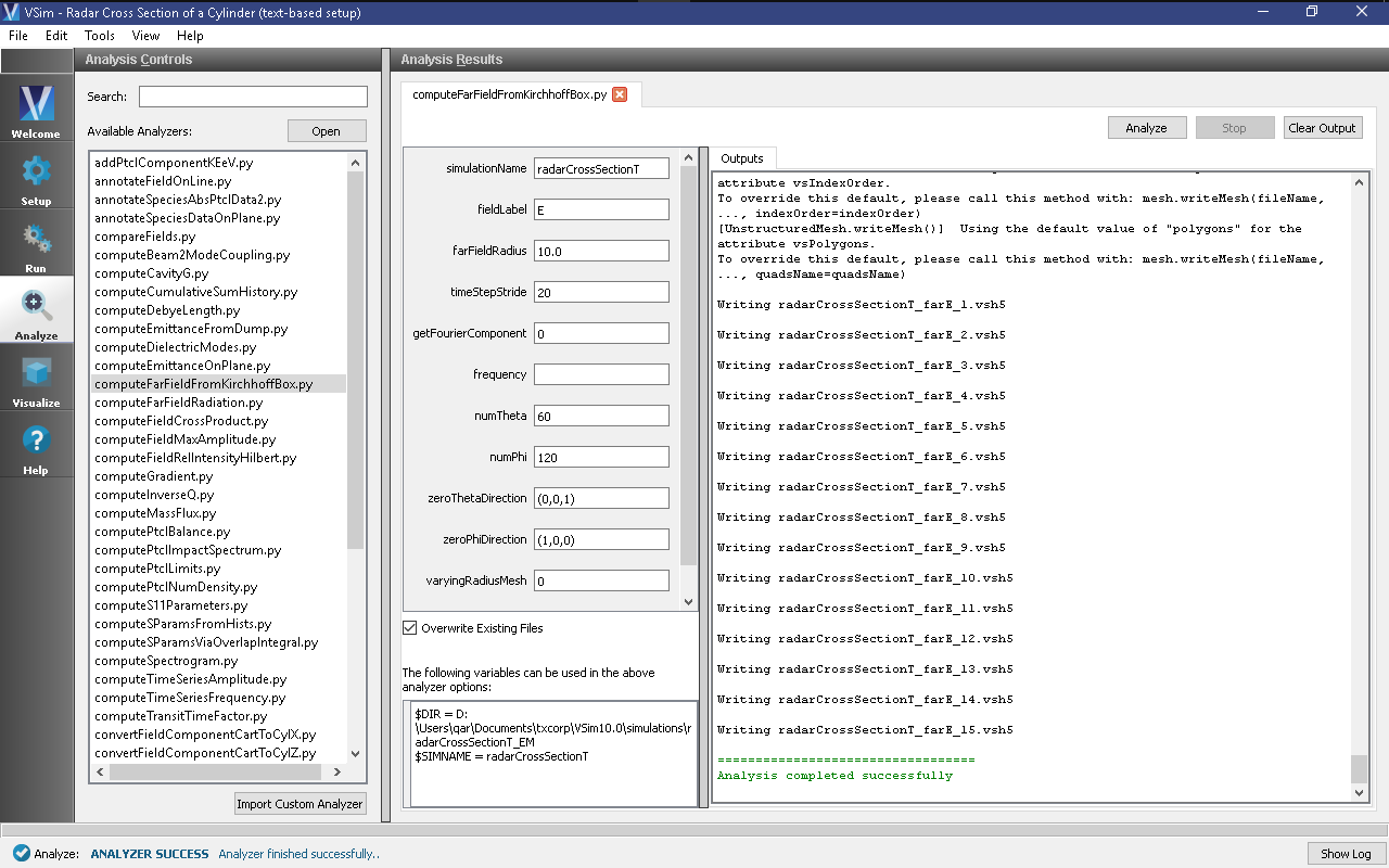
Fig. 286 The Analysis Window after running
Visualizing the Results
After performing the above actions, proceed to the Visualize Window by pressing the Visualize button in the left column of buttons.
The Radar cross section as shown in Fig. 287, do the following:
- Expand Scalar Data
- Select farE
- Expand Geometries
- Select farSphere
- Select poly
- Select Clip All Plots
You should see the far field, time-dependent signal on the sphere with the cylinder in the center.
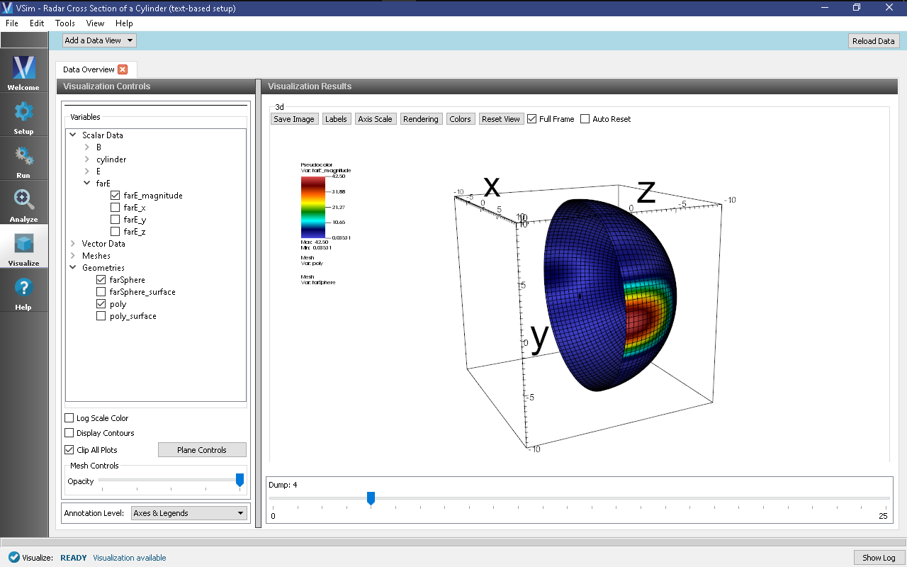
Fig. 287 The radar cross section
Further Experiments
The physical dimensions of the cylinder can be modified from the parameters window.