Argon Plasma (ArPlasmaT.pre)
Keywords:
- global simulation, gas
Problem Description
Description of simulation here…..
This simulation can be run with a GSimPlasma license.
Opening the Simulation
The Argon Plasma example is accessed from within GSimComposer by the following actions:
Select the New → From Example… menu item in the File menu.
In the resulting Examples window expand the GSim for Plasmas option.
Expand the NobleGasesT option.
Select Argon Plasma and press the Choose button.
In the resulting dialog box, create a New Folder if desired, then press the Save button to create a copy of this example.
The resulting Setup Window is shown in arplasmasetupwin.
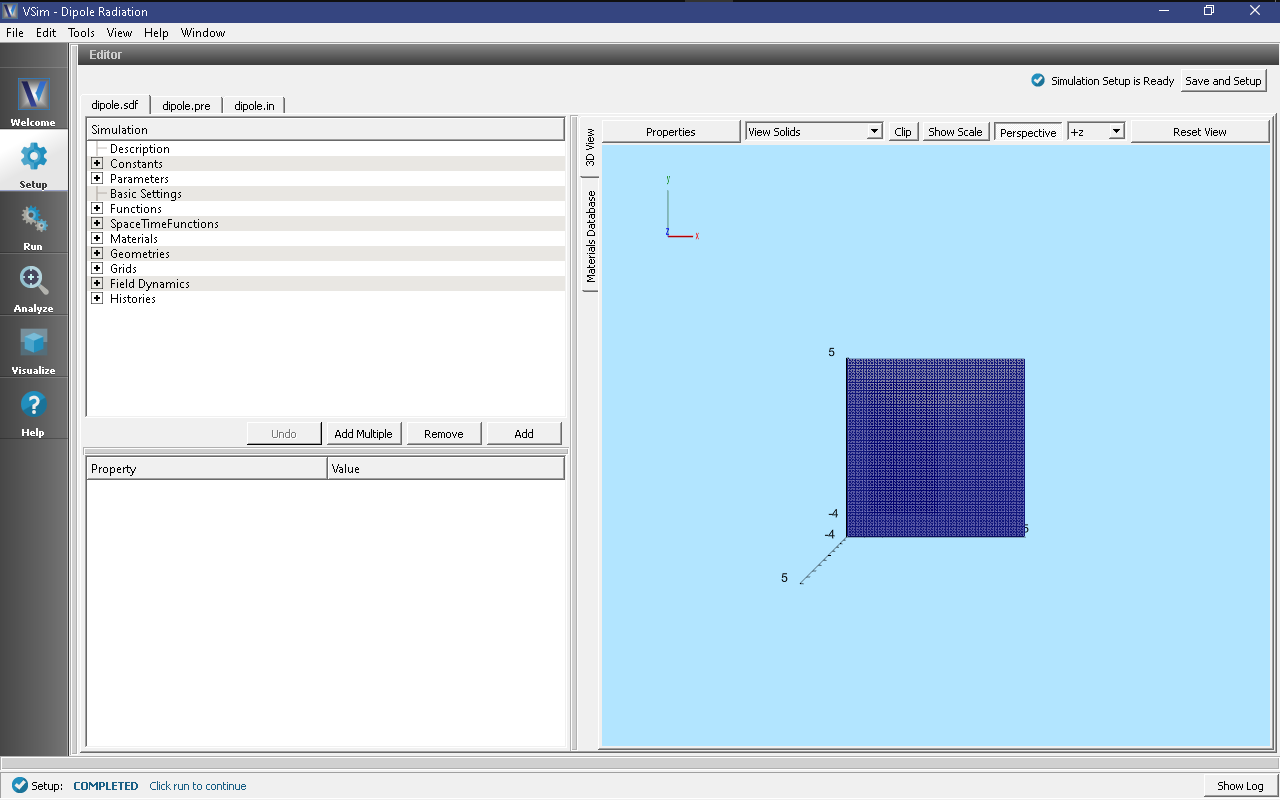
Setup Window for the Dipole example.
Running the Simulation
To run the simulation:
Proceed to the run window by pressing the Run button in the left column of buttons.
Here you can set run parameters, including how many cores to run with (under the MPI tab).
When you are finished setting run parameters, click on the Run button in the upper left corner. You will see the output of the run in the right pane.
The run has completed when you see the output, “Engine completed successfully.”
This is shown in arplasmarunwin. The number of steps chosen in this
run is sufficient so that the radiation reaches the Kirchoff box and the field histories
are recorded for a sufficient duration.
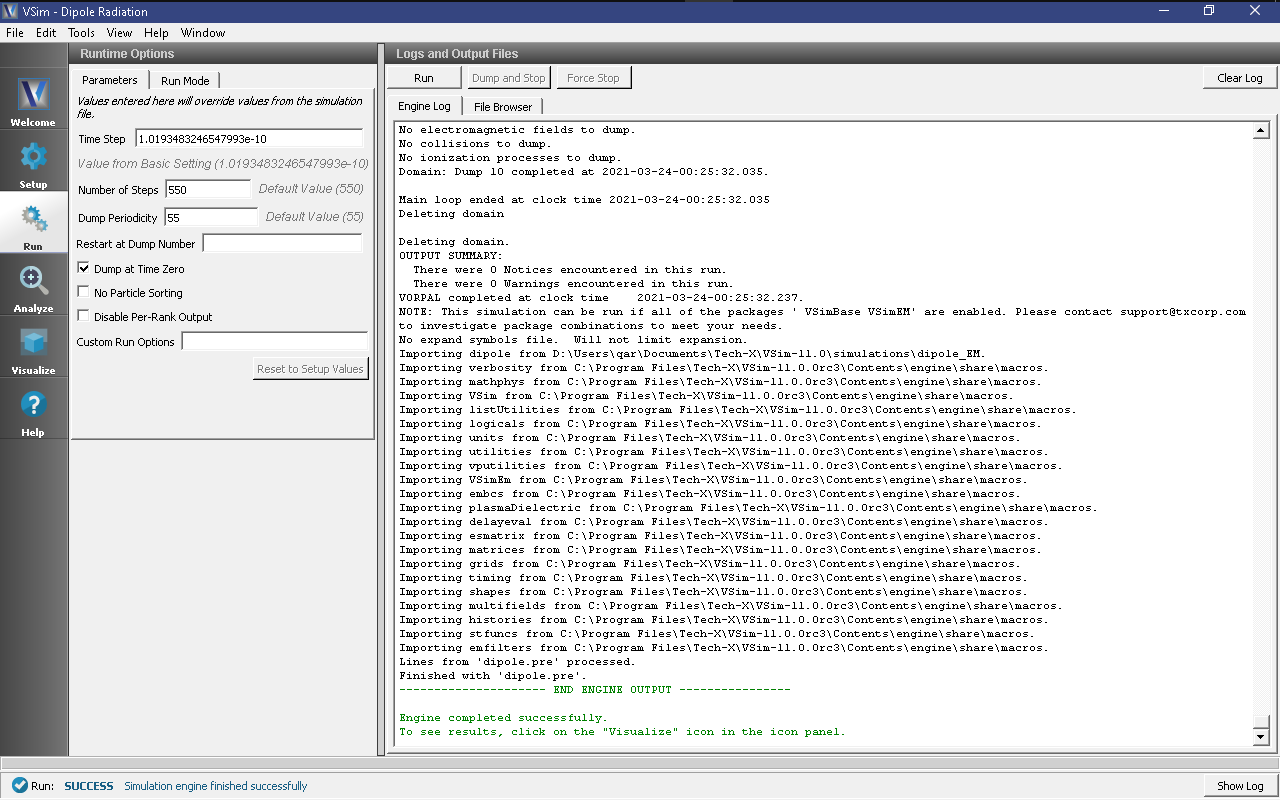
The Run window at the end of execution.
Running the Analyzer
After completing the run, one can run the analyzer to compute field values at far away points. To bring up the analyser script, Click on the Analyze icon. The panel that appears will be named computeFarFieldFromKirchoffBox.py, along with a set of text boxes in which the necessary parameters need to be filled. For the defailt settings of the file you may use the following:
simulationName - ArPlasmaT
fieldLabel - E
farFieldRadius - 1024.0
numPeriods - 0.25
numFarFieldTimes - 2
frequency - 0.3e9
numTheta - 17
numPhi - 17
zeroThetaDirection - (0,1,0)
zeroPhiDirection - (0,0,1)
incidentWaveAmplitude - blank
incidentWaveDirection - (0,0,0)
varyingMeshMaxRadius - 1024.0
principalPlanesOnly - checked
Note that some entries need to be left blank.
After entering the above parameters, also shown in
arplasmaanalyzewin, press the “Analyse” button
that appears on the upper right side.
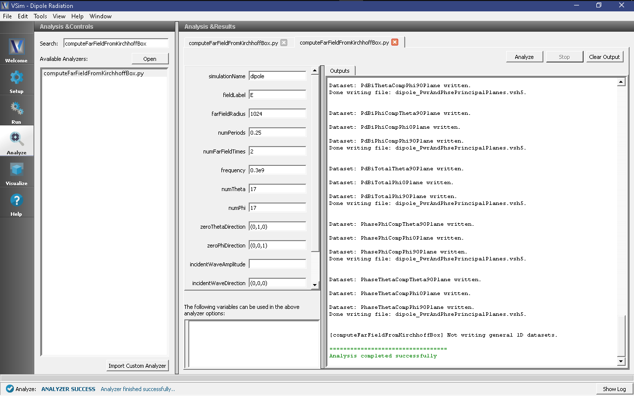
The Analyze Window at the end of analyzer execution.
Visualizing the Results
After performing the above actions, the results can be visualized as follows:
Proceed to the Visualize Window by pressing the Visualize button in the navigation column.
With the Add a Data View expanded, click on Field Analysis.
In the Visulaization Controls section, expand the Field menu and click on farE_magnitude.
Choose X-Intercept in the Slice settings, and choose 3d Only in Layout.
Use the mouse to orient the torus as shown in arplasmavizwin.
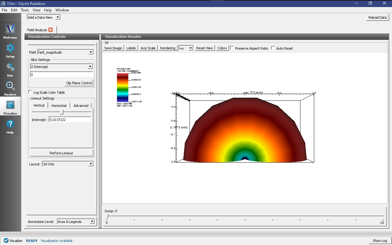
The magnitude of the electric field is propotional to the time averaged power flux.
Further Experiments
Change some of the parameters such as ………… in the set up window to see a variation in the …………