Argon Plasma (ArPlasmaDynSheath.sdf)

Keywords:

global simulation, gas, reaction rates

Problem Description

This simulation models chemical reactions that occur in an Argon plasma at low pressure. The model allows users to input a specified power and chamber size. This model also includes a sheath boundary condition to correctly account for the behavior of charged particles at a sheath. GSim computes steady state densities, temperatures, and reaction rates.

This simulation can be run with a GSimPlasma license.

Opening the Simulation

The Argon Plasma example is accessed from within GSimComposer by the following actions:

• Select the New → From Example… menu item in the File menu.

• In the resulting Examples window expand the GSim for Plasmas option.

• Expand the NobleGases option.

• Select Argon Plasma and press the Choose button.

• In the resulting dialog box, create a New Folder if desired, then press the Save button to create a copy of this example.

The resulting Setup Window is shown in arplasmasetupwin.

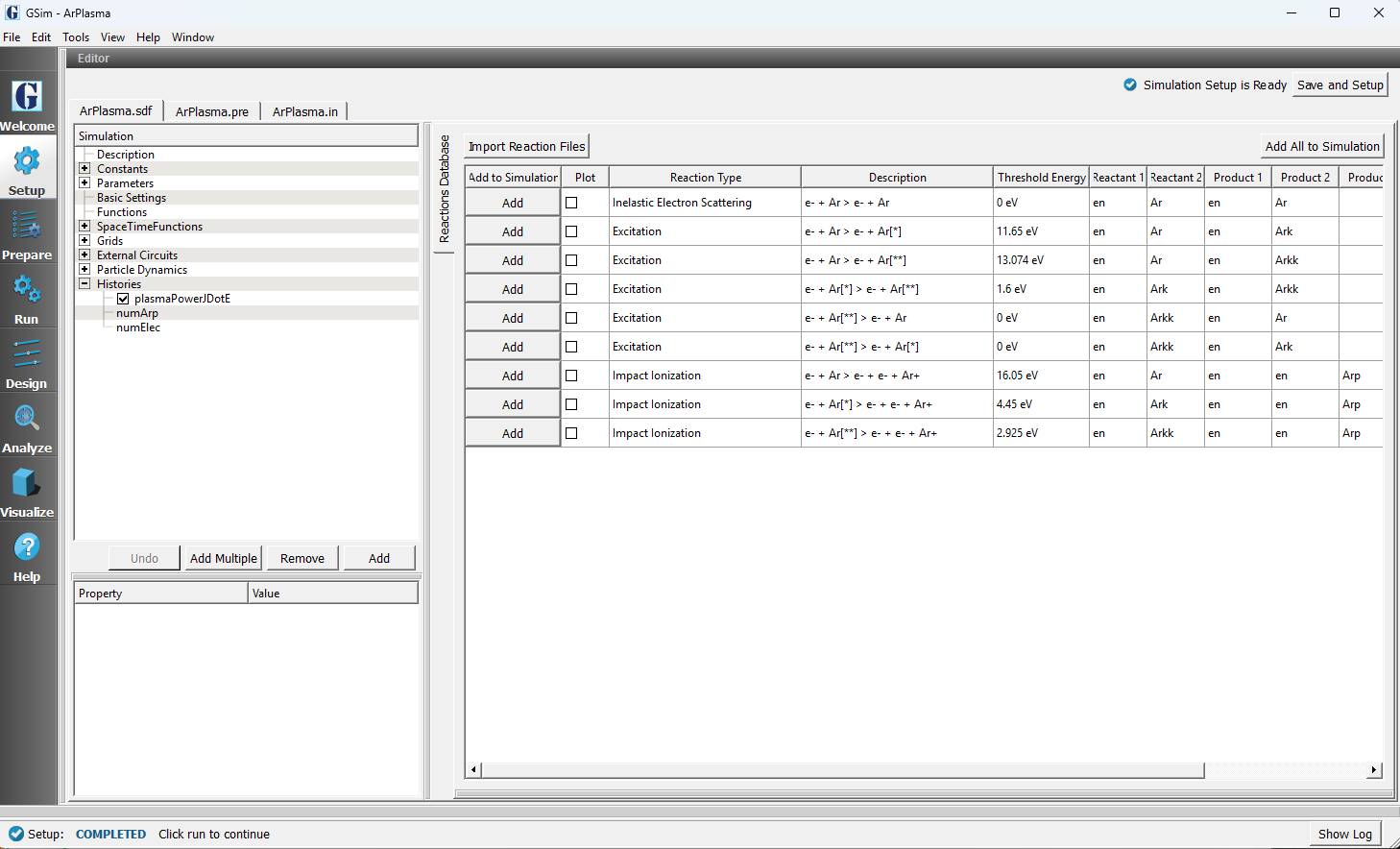
Setup Window for the argon plasma dynamic sheath example.

Basic Simulation Concepts

GSim is a kinetic global simulation that is able to predict the dominant reactions that are important when considering a specific chemistry. GSim can also predict steady state plasma and neutral densities. These can be useful when initializing complex reaction scale models of CCP and ICP chambers. GSim applies an out-of-plane electric field in the z-direction. The power is specified by the user and feedback on the plasma J dot E power is used to maintain constant power. The in-plane electric field is computed via Gauss’ law. From this in-plane electric field, we then compute the sheath voltage. Finally, we have developed a “zero-width” sheath model which uses the sheath voltage to reflect low energy electrons and absorbs high energy (tail) electrons which can overcome the sheath potential.

Key parameters used in this simulation that the user could consider modifying.

• POWER: RF averaged power of external drive

• NEUTRAL_PRESSURE_Torr: Neutral pressure in Torr

• RF_FREQ: Frequency of external power source

Running the Simulation

To run the simulation:

• Proceed to the run window by pressing the Run button in the left column of buttons.

• When you are finished setting run parameters, click on the Run button in the upper left corner. You will see the output of the run in the right pane.

The run has completed when you see the output, “Engine completed successfully.” This is shown in arplasmarunwin. The number of steps chosen in this run is sufficient to reach steady state.

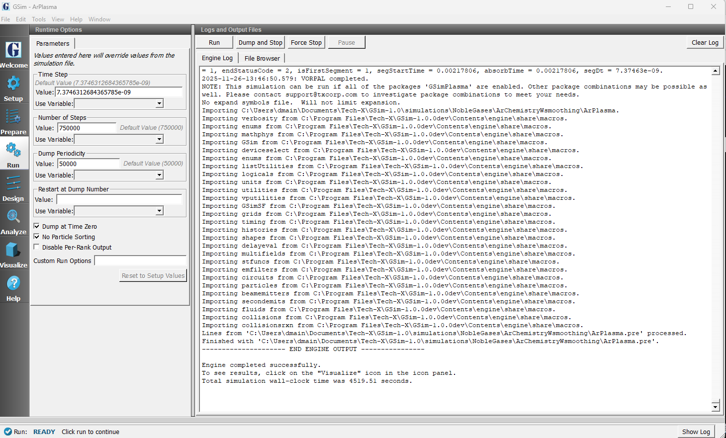
The Run window at the end of execution.

Setting up the sheath electric field

The out-of-plane electric field and sheath electric field are both set up in basic settings. We have two methods to model the sheath potential. In this example, we are dynamically computing the electric field which is solved via Gauss’ law. We then self-consistently compute the electron Debye length (\(\lambda_{De}\)) based on the electron temperature and density, but of which are calculated at each time step. Finally, the sheath potential is found via

\(V_{sheath} = E_{sheath}*\lambda_{De}\)

The other method of modeling the sheath potential is by assuming a fixed sheath potential that does not evolve.

In Basic Settings, the user also specifies the “drive electric field”. In this example, the drive electric field has been chosen by right clicking next to “drive electric field” under “sheath type” in Basic Setting. We have created a SpaceTimeFunction called “EzofTime”, which we have chosen to use for this example. “EzofTime” is a 13.56 MHz sinusoidal wave form. Figure arplasmabasicsettings shows how to access the sheath settings and the location within Basic Settings.

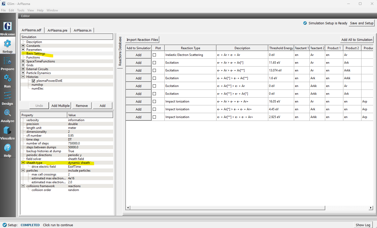
The setup window showing how to set up the sheath model in Basic Settings.

Creating the Constant Power Source

The constant power source is set up under External Circuits in Composer. To create a constant power source, right click on “External Circuits” and choose “Add Specified Power Current Source”. This create a new option called “constantPowerCircuit0”. Double click on “constantPowerCircuit0” and choose a new name if you would like. We have called the constant power block “plasmaPower”. The input parameters are “power profile”, “filter time constant”, and “relative notch filter width”. We have input a STFunc for the power profile. The filter time constant specifies a relaxation time scale for smoothing over particle noise. Finally, the relative notch width filter is the width of a band notch filter we have implemented to subtract out the RF signal in the plasma power.

Setting up Plasma Properties

The plasma is enabled under Basic Settings. To do this, click on Basic Setting. Then in the Property box (below Basic Settings), click in the region next to “particles” and choose “include particles”. Then under “collisions framework”, choose “reactions”. These options have already been chosen for this example. Choosing these options creates a “Particle Dynamics” tab in Composer. To examine the properties of the plasma, first expand the Particle Dynamics tab, then expand the “KineticParticles” tab. Finally expand “electrons” and “Arp” to examine the initial conditions for the two kinetic species. The initial condition for each species is a Maxwellian distribution with a specified initial temperature. The boundary condition is fixed in GSim. Although the user can change the boundary conditions, we do not suggest the user add any particle boundary conditions. On the right boundary at XMAX, the particles reflect. On the left boundary, ions are absorbed. Electrons are absorbed if the energy is greater than the sheath potential and reflected if the energy is less than the sheath potential.

This simulation includes 3 fluids: ground state Ar, and two excited states. Both excited states are assumed to be metastable states and thus contribute to the plasma discharge. To examine the reactions in this example, expand “Reactions” then expand “Particle Fluid Collisions”. Here you will see 11 reactions that have been included in this simulation. The names of each reaction is identical to the name of the cross section table. We require this naming scheme to simplify the post processing routines written for GSim.

Running the Analyzer

After completing the run, the user can compute the reaction rates. To do this, navigate to the “Analyze” option. Then click on “computeRxnRate.py”. This analyzer has already been selected with the following input parameters

• simulationName - ArPlasmaDynSheath

• dumpTimei - 0

• dumpTimef - 20

• Timei - 6e-3

• Timef - 7e-3

“dumpTimei” and “dumpTimef” are the first and last dump numbers. “Timei” and and “Timef” are the beginning and ending times to compute the reaction rates. The chosen times corresponds to times the plasma is in steady state. After populating the required parameters, press the “Analyze” button that appears on the upper right side. Figure arplasmaanalyzewin shows the analyze window as it appears in GSim.

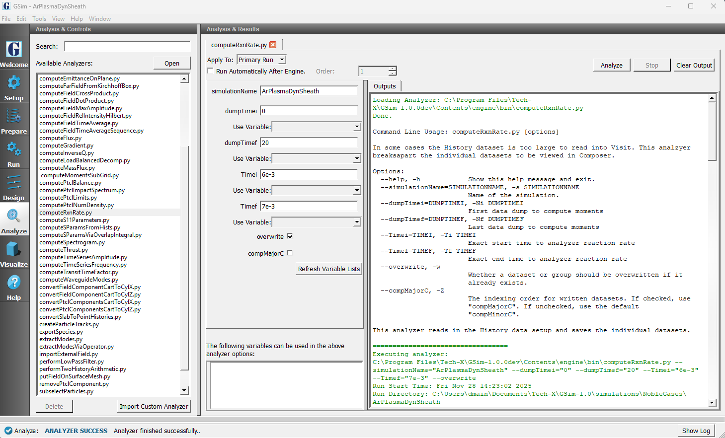
The Analyze Window at the end of analyzer execution.

The reaction rates for this simulation are shown in Figure arplasmaRxnRates1 and arplasmaRxnRates2. The reaction rates are broken into two plots called ArPlasmaDynSheath_ReactionRate1.png and ArPlasmaDynSheath_ReactionRate2.png. For an Argon plasma, all the rates would fit on one plot. However, for more complex plasmas two or more plots are needed.

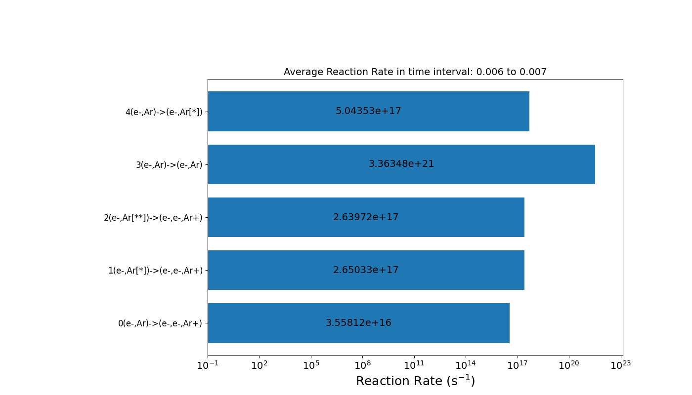
First half of reactions rates from the simulation.

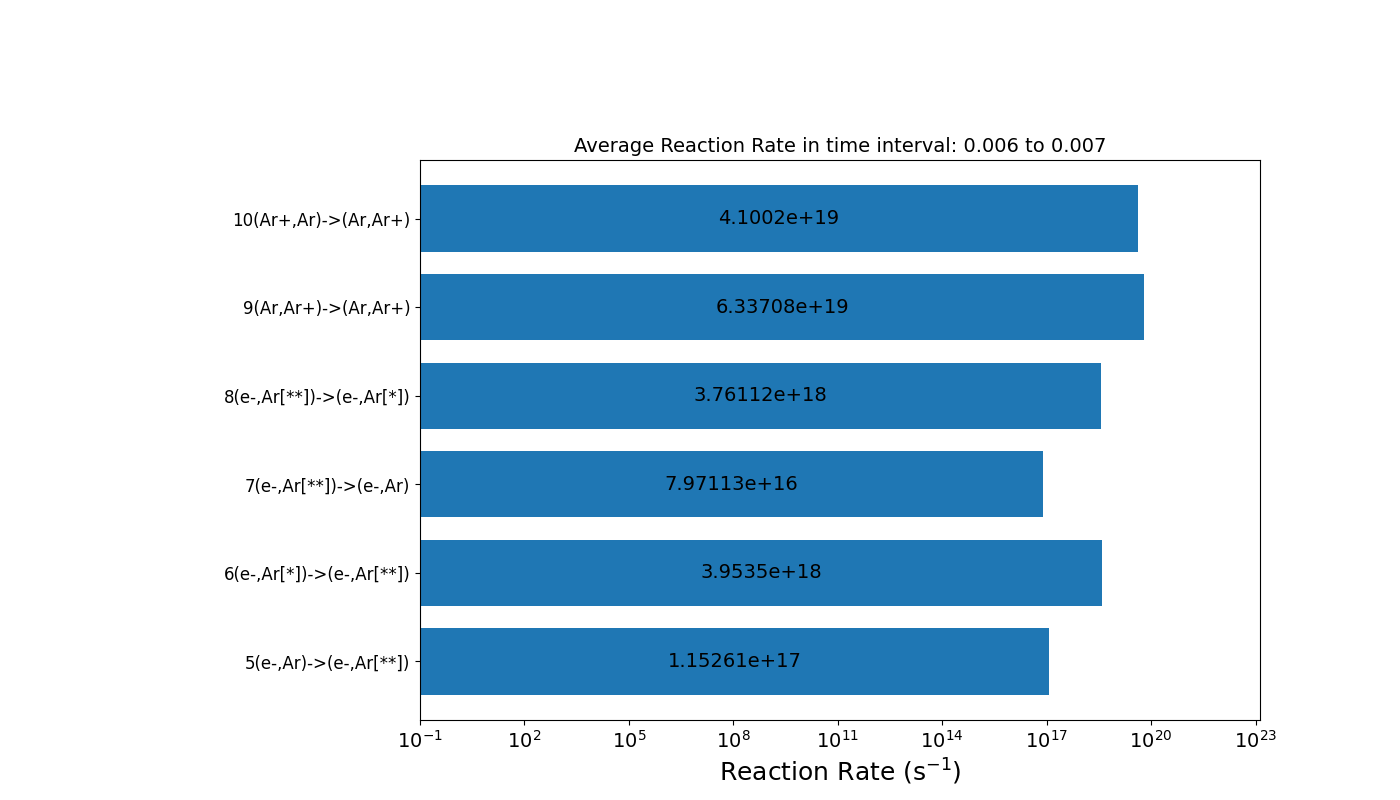
Second half of reactions rates from the simulation.

In addition to the reaction rates, the analyzer also plots the fluid density. For this example, the plot of fluid density is called ArPlasmaDynSheath_FluidDensity.png. One more analyzer that you may find useful is called computeMomentsSubGrid.py which subdivides the grid into a user specified number of sub-grids and computes the density, flow velocity, and temperature as a function of position at each saved data dump using particle data.

Visualizing the Results

After performing the above actions, the results can be visualized as follows:

1. Proceed to the Visualize Window by pressing the Visualize button in the navigation column.

2. With the Add a Data View expanded, click on History.

3. In the Visulaization Results section, click on Add Curve and choose “electronTempIneVHist”.

The above steps plots a history of the electron temperature. The physical number of electrons has already been plotted and pre-loads when you click on the “Visualize” option. The number of physical electrons and ions are shown in Figure arplasmavizwin. The volume of the chamber is given by \(V = LX * LY * LZ\) = 0.05 m. This is found by noting that LX = 0.05 m, LY = 1.0 m and LZ (which is the unsimulated dimension) is 1.0. Therefore from Figure arplasmavizwin we see that the steady state electron and ion density is about \(1.8 \times 10^{16}\) m \(^{-3}\).

History showing the number of physical electrons and ions.

Further Experiments

Further experiments include changing the input power. Other simulations may include changing the volume of the domain.