Scattering off a Metal Sphere with a Dielectric Coating (dielecCoatedMetalSphere.sdf)

Keywords:

Mie Scattering Dielectric Coated Metal Sphere

Problem description

The example describes the scattering of electromagnetic waves off a metal sphere with a dielectric coating, which is a modification of the previous example that described scattering off a pure metal sphere.

An incident plane wave is launched toward the sphere. XSim computes the resulting fields in the vicinity of the sphere, within a computational domain by applying the proper boundary conditions around the surface of the sphere. The waves that exit the computational domain are absorbed into MAL layers.

The fields for points far away from the sphere, beyond the computational domain, are computed with the help of an analyzer that is part of the XSim distribution. The histories of the electric and magnetic fields are recorded along a closed surface known as a Kirchhoff box that lies near the simulation domain edge and before the MAL layers. This field information is then used to compute fields far away from the sphere center by applying the Kirchhoff integral theorem.

In this example, the radius of the metal sphere is set to equal 0.3367m and the wavelength is nearly 1m at 0.99931m. The thickness of the coating is 0.1 times the wavelength. The computational domain extent is set to three times the wavelength in all directions along the three coordinate axes. The thickness of the MAL layer is twice the wavelength. The resolution of the grid corresponds to 24 cells per wavelength. This parameter is chosen such that the thickness of the dielectric layer is resolved. The time step is chosen to be very close to the Courant condition limit. The wave is launched from the positive \(z\) direction, and the incident wave electric field is polarized along the \(x\) direction. Care needs to be taken so that the simulation is performed for a sufficient number of time steps, so that the wave reaches the surface of the Kirchhoff box where the histories are recorded. Thus, changing the frequency or the resolution of the grid would alter the time step, and the number of steps required to complete the run will need to be changed accordingly.

Opening the Simulation

The Mie Scattering, Dielectric Coated Metal Sphere example is accessed from within XSimComposer by the following actions:

• Select the New → From Example… menu item in the File menu.

• In the resulting Examples window expand the XSim for Electromagnetics option.

• Expand the Scattering option.

• Select “Scattering off a Metal Sphere with a Dielectric Coating” and press the Choose button.

• In the resulting dialog, create a New Folder if desired, and press the Save button to create a copy of this example.

All of the properties and values that create the simulation are now available in the Setup Window as shown in Fig. 308. You can expand the tree elements and navigate through the various properties, making any changes you desire. The right pane shows a 3D view of the geometry, if any, as well as the grid, if actively shown. To show or hide the grid, expand the Grid element and select or deselect the box next to Grid. While the setup is similar to the previous example of a pure metal sphere, the additional components in this example may be found as follows: Expand the Menu under Material to see the element COATING. As showed in Fig. 308, clicking on COATING shown the properties of the dielectric material. In addition, expand the menu under Geometries, followed by the menu under CSG to see the additional geometry element, coating.

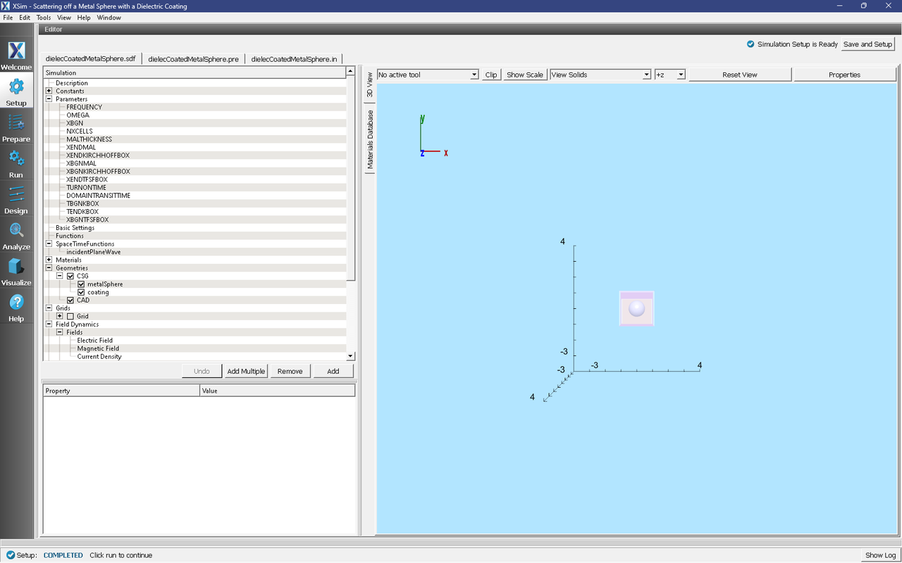
Fig. 308 Setup Window for the Mie Scattering example.

The Setup Window shows the Kirchhoff box, with the metal sphere at the center. To see the grid, click on the drop down menu of “Grids” on the left side panel. Check the box beside “Grid”. In order to view or change the wave frequency, click on the drop down menu “Parameters” and then click on “Frequency”. To view or change the direction of the incident wave or polarization, you can click on the drop down menu “Field Dynamics”, then the drop down menu “RCSBox”. Following this, check the box beside “rcsBox0”. The lower left panel displays a table with the wave property and its corresponding value.

Running the simulation

After performing the above actions, continue as follows:

• Proceed to the run window by pressing the Run button in the left column of buttons.

• Check that you are using these run parameters:

  • Time Step: 3.8115448780607225e-11

  • Number of Steps: 4000

  • Dump Periodicity: 200

  • Dump at Time Zero: Checked

• Click on the Run button in the upper left corner of the right pane.

You will see the output of the run in the right pane. The run has completed when you see the output, “Engine completed successfully”. This result is shown in Fig. 309.

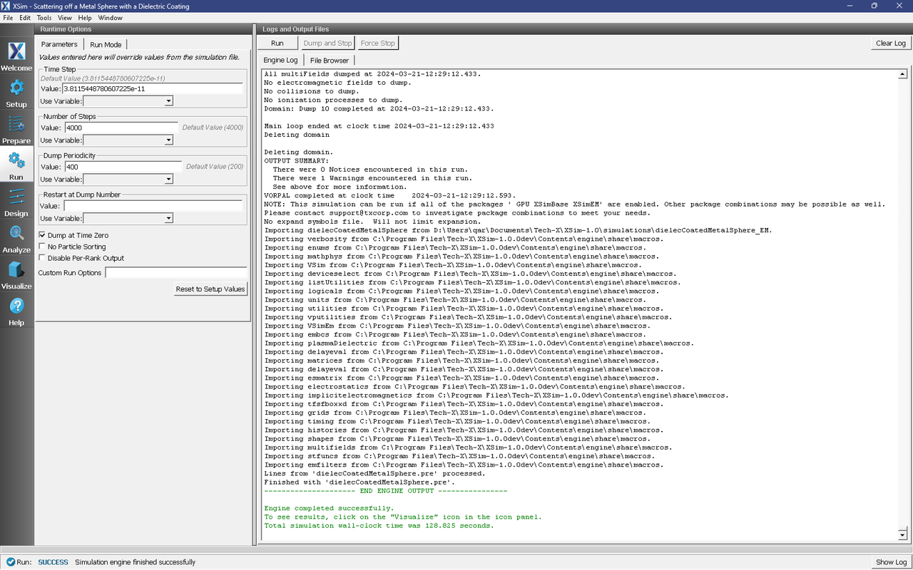
Fig. 309 The Run Window at the end of simulation.

Running in 3D, this simulation uses around 4000 time steps. The run takes about 15 minutes on a 4-core 2.3 GHz processor.

Running the Analyzer

After completing the run, one can run the analyzer to compute field values at far away points. To bring up the analyser script, Click on the Analyze icon. The panel that appears will be named computeFarFieldFromKirchhoffBox.py, along with a set of text boxes in which the necessary parameters need to be filled. For the default settings of the file you may use the following:

• simulationName : dielectricCoatedMetalSphere

• fieldLabel : E

• farFieldRadius : 50.0

• backgroundEpsRel : 1.0

• numPeriods : 0.25

• numFarFieldTimes : 2

• frequency : 0.3e9

• numTheta : 31

• numPhi : 64

• zeroThetaDirection : (0,0,1)

• zeroPhiDirection : (1,0,0)

• incidentWaveAmplitude : 1.0

• incidentWaveDirection : (0,0,1)

• varyingMeshMaxRadius : 1

• principalPlanesOnly : checked

After entering the above parameters, also shown in Fig. 310, press the “Analyze” button that appears on the upper right side.

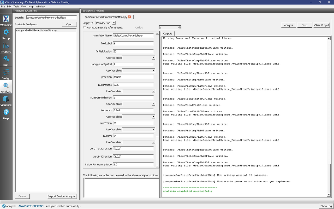
Fig. 310 The Analyze Window at the end of analyzer execution.

Visualizing the results

After performing the above actions, click on Visualize in the column of buttons at the left. The program will load the data and provide you with certain options.

One of the quantities that is of interest in such scattering phenomena is radar cross section (RCS) measured in dBsm. The RCS, sometimes designated as \(\sigma\), having units of \(m^2\), is given as

\[RCS = 4 \pi R_s^2 \frac{P_r} {P_i}\]

where \(R_s\) is the radial distance from scatterer, \(P_r\) is the power flux received at the point of interest, and \(P_i\) is the incident power flux. In MKS units the power flux is measure in \(W/m^2\). RCS in dBsm is given as

\[10log_{10}(RCS)\]

To obtain plots of this quantity, click on the drop down menu, Add a Data View. In this menu, choose 1-D Fields. Then click the Add Curve button. Select the Variable drop-down menu and select PdBsmTotalPhi0Plane. Then select Add Window, then the Add Curve button on that window. Select the Variable drop-down menu and choose PdBsmTotalPhi90Plane. The resulting plots are shown in Figure Fig. 311.

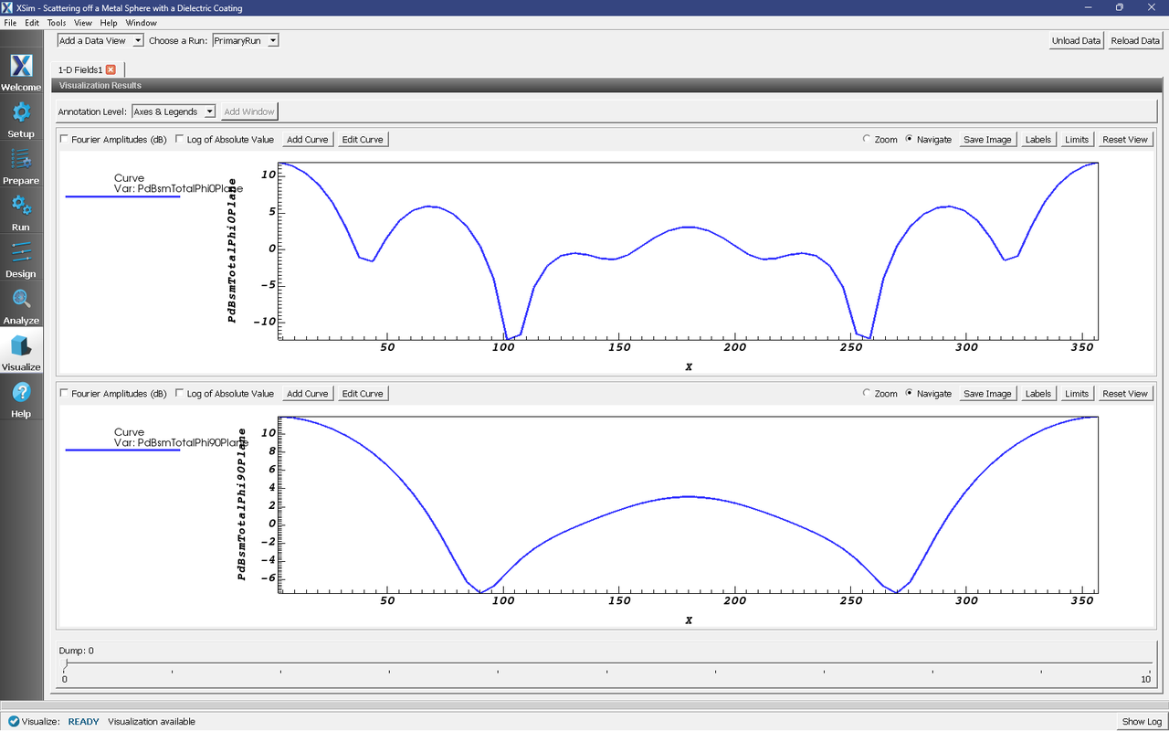
Fig. 311 The Visualize Window at the end of execution.

Further Experiments

Alter the thickness or the dielectric constant of the coating to see its effect on the computed RCS.