Colliding Pulse Injection (collidingPulseInjT.pre)

Keywords:

laser plasma accelerator, controlled injection, colliding laser pulses

Problem description

This example demonstrates the use of VSim to simulate controlled injection in a laser-plasma accelerator using colliding laser pulses [CMRB+10]. Two laser pulses are launched from opposite sides (one from the left side and the other one from the right side of the box) and propagate in opposite directions. The laser pulse coming from the left side is the main pulse that drives the plasma wake. The laser pulse coming from the right is the collider pulse, with much lower intensity than the main pulse. It can also propagate with a small angle with respect to the main pulse propagation axis. When the two lasers collide they create a slow beat wave, which allows electrons of the background plasma to be trapped and be accelerated by the wakefield driven by the main pulse.

In this example, the laser pulses are polarized in the \(y\) direction and both have a Gaussian profile defined by

\[E_y = E_{\rm pump\_(L,R)} \exp(- x^2/{\rm LPUMP\_ (L,R) }^2) \exp(-(y^2 + z^2)/ {\rm W0\_(L,R)}^2)\]

where L and R refer to the left and right pulse respectively. The laser intensity is defined through the normalized vector potential

\[{\rm APUMP\_(L,R)} = e E_{\rm pump\_(L,R)}/\omega_{\rm (L,R)} m_e c\]

where \(\omega = 2\pi c /{\rm WAVELENGTH\_(L,R)}\) is the laser frequency.

The pulses enter a plasma channel with density on axis DENSITY0 through a density ramp of length 20 \(\mu\) m.

This simulation can be performed with the VSimPA or VSimPD license.

Opening the Simulation

The Colliding Pulse Injection example is accessed from within VSimComposer by the following actions:

• Select the New → From Example… menu item in the File menu.

• In the resulting Examples window expand the VSim for Plasma Acceleration option.

• Expand the Laser Driven Acceleration (text-based setup) option.

• Select Colliding Pulse Injection (text-based setup) and press the Choose button.

• In the resulting dialog, create a New Folder if desired, and press the Save button to create a copy of this example.

The basic variables of this problem can now be changed via the text boxes in the left pane of the Setup Window, as shown in Fig. 491.

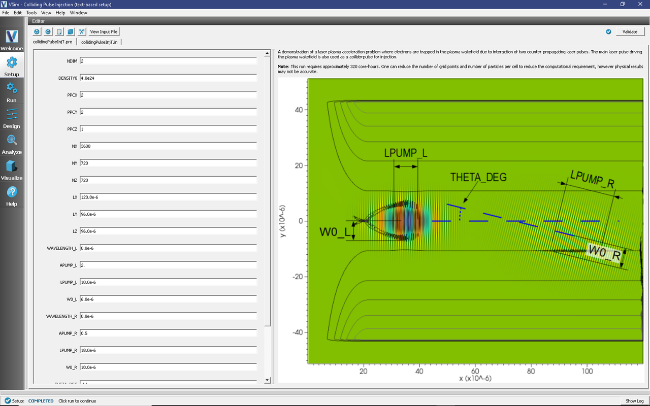
Fig. 491 Setup Window for the Colliding Pulse Injection example.

Input File Features

The simulation setup consists of an electromagnetic solver using the Yee algorithm. Two laser launchers are used, one from the left edge and the other from the right edge of the window. PMLs are used on the transverse sides of the window to absorb outgoing waves. The plasma is represented by macroparticles which are moved using the Boris push. The particles are variably weighted to represent the density ramp, and they have a unique tag. The current deposited by the particles is smoothed using four passes of the 1-2-1 filter and subsequently applying a compensator.

The input file allows one to set up both lasers, plasma and grid parameters.

Running the Simulations

Running in 2D, this simulation uses around 2,600,000 cells and nearly \(10^7\) particles. This run requires about 320 core-hours for the full 156,000 steps on a 2.5 GHz I7. On less powerful hardware, one can reduce the number of steps to 15000 see just the collision or one can reduce the number of grid points and number of particles per cell to see more of the evolution, but physical results may not be accurate.

To run on local hardware do

• Proceed to the Run Window by pressing the Run Tab in the left column of buttons.

• Set the number of steps to 5000 and the dump periodicity to 500 in order to see the initial evolution. The collision occurs at step 4500 (dump 9).

• Run in parallel with as many physical cores as are on your machine, because this is a computationally intense problem. Even with the reduced number of steps, this run can take up to 7 hours on four cores for 5000 steps, depending on the processor.

• To run the file, click on the Run button in the upper left This is shown in Fig. 492. The run has completed when you see the output, “Engine completed successfully.” in this same pane.

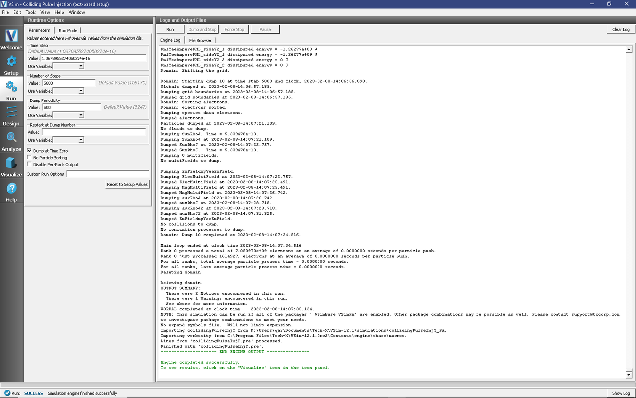
Fig. 492 The Run Window.

Alternatively, copy collidingPulseInjT.pre to your more powerful hardware and run it through the command line or submit it to your job queue.

Visualizing the Output

If you have run the job on a remote computer, you would now need to copy back the files that you want to visualize locally into the local directory in which one has the input file open. E.g.,

for dmpnum in 0 8 9 10; do
  scp mybigcomputer.mydomain:myspace/collidingPulseInjT_*_${dmpnum}.h5 .
done

Then proceed to the Visualize Window by pressing the Visualize button in the left column of buttons.

• To view the transverse electric field, switch to the Data Overview in the Visualization Controls pane.

• Under Visualization Controls, Variables, From the Field drop down menu, choose the y component of the ElecMultiField.

• Set the color scale by checking the Set Minimum and Set Maximum boxes in the Color Table subwindow under Visualization Controls. Then set the minimum to -2e12 and the maximum to 2e12.

• Click the Auto Reset check box.

• Move the dump slider to position 8, then 9, then 10 to see the pulses collide.

The collision of the pulses is then seen as shown in Fig. 493 below.

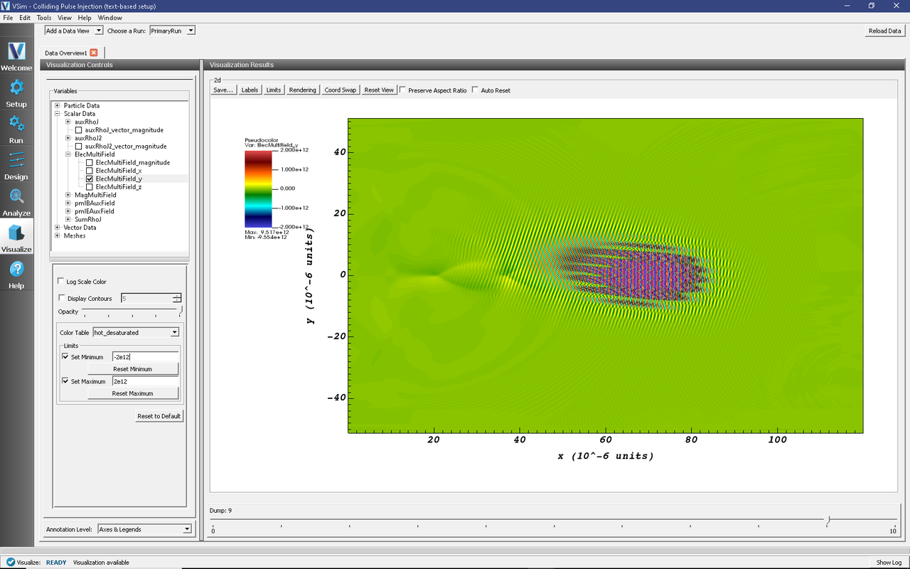
Fig. 493 Visualization of the transverse electric field as a color contour plot and longitudinal lineout.

The x-component shows the wake field of the left incoming pulse and some of the electromagnetic field of the incoming collider pulse. The wake field can be better seen by clicking on the Colors button and setting the min and max to be -+ 1.e11. The plasma density can be seen in the zeroth component of the SumRhoJ field.

Particle phase-space can be seen by switching to the Phase Space Data View in the Controls pane. Fig. 494 shows the particle longitudinal momentum as a function of the longitudinal coordinate just after the collision.

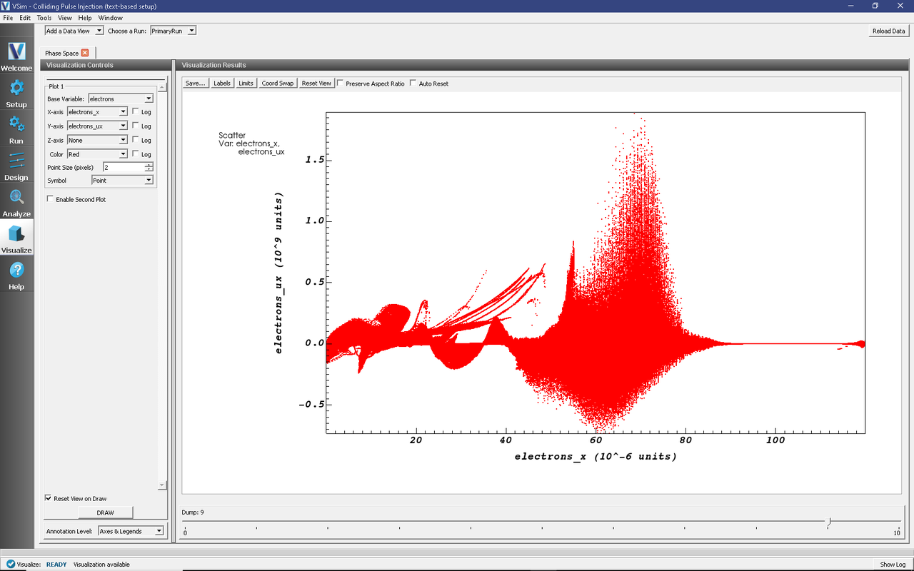
Fig. 494 Visualization of the particle longitudinal phase-space during collision. Particles kicked up into the trapped region by the colliding pulses. One can see the acceleration of particles to high energy in later dumps.

Continuing the simulation

The simulation to this point has allowed one to study the initial injection of particles up to high energy, so that they can be trapped by the wake. One can now continue this simulation to study the acceleration in the wake. Since this simulation stopped at dump 10, one can now set the additional Runtime Options to unclick Dump at Time Zero and then set Restart at Dump Number to 10. Since at this point, the evolution changes more slowly, one can set the Number of Steps to 10000 and the Dump Periodicity to 5000. Again hit Run.

At any time one sees that another data dump has occurred, one can switch over to the Visualize pane and hit Reload Data to view the new available data, any of the fields or particles as before.