Laser Ionization (laserIonization.sdf)
Keywords:
- electromagnetic, particle in cell, field ionization, moving window
Problem description
This example launches an electromagnetic laser pulse into a homogeneous volume of neutral argon gas. The field strength is significant enough to ionize the argon to multiple ionization states, which are included in the simulation. The neutral gas density is depleted as the ionization occurs, with layers of argon atoms at increasing ionization levels towards the center of the Gaussian beam.
This simulation can be performed with a VSimPD license.
Opening the Simulation
The Laser Ionization example is accessed from within VSimComposer by the following actions:
Select the New → From Example… menu item in the File menu.
In the resulting Examples window expand the VSim for Plasma Acceleration option.
Expand the Laser Driven Acceleration option.
Select “Laser Ionization” and press the Choose button.
In the resulting dialog, create a New Folder if desired, and press the Save button to create a copy of this example.
All of the properties and values that create the simulation are now available in the Setup Window as shown in Fig. 483. You can expand the tree elements and navigate through the various properties, making any changes you desire. The right pane shows a 3D view of the geometry, if any, as well as the grid, if actively shown. To show or hide the grid, expand the Grid element and select or deselect the box next to Grid.
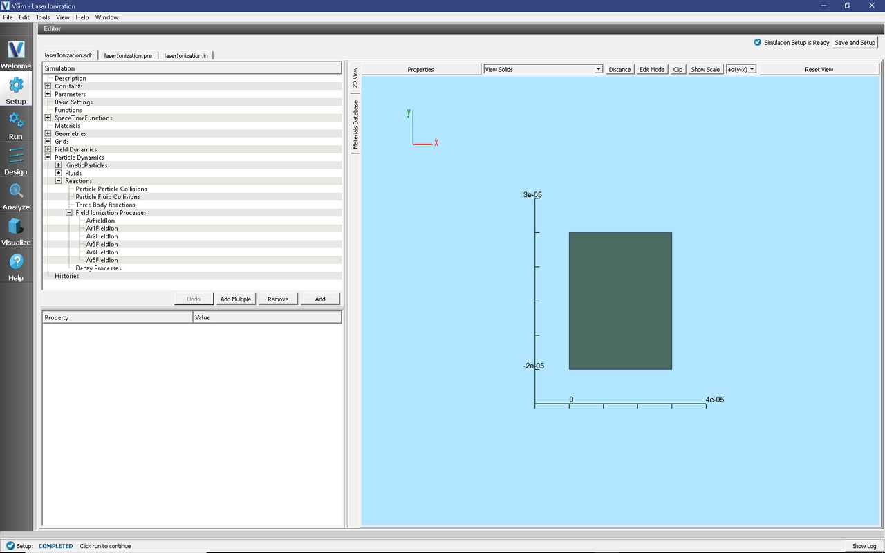
Fig. 483 Setup Window for the Laser Ionization example.
Simulation Properties
Constants are set up to allow setting the laser amplitude and the neutral argon density (1/m^3).
Running the Simulation
After performing the above actions, continue as follows:
Proceed to the Run Window by pressing the Run Tab in the left column of buttons.
To run the file, click on the Run button in the upper left corner of the Logs and Output Files pane. You will see the output of the run in the right pane. The run has completed when you see the output, “Engine completed successfully.” A snapshot of the simulation run completion is shown in Fig. 484.
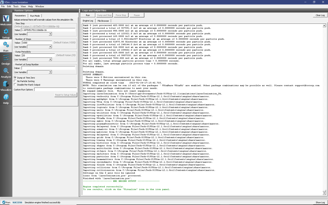
Fig. 484 The Run Window at the end of execution.
Visualizing the Results
After performing the above actions, continue as follows:
Proceed to the Visualize Window by pressing the Visualize Tab in the left column of buttons.
View the electric field magnitude, by doing the following:
Expand Scalar Data, expand E and select E_magnitude.
Scrolling through time (by moving the slider at the bottom of the window) will show the laser pulse propagating across the simulation domain.
It may be useful to check the Auto Reset button in the 2d plot.
Next, untick the E_magnitude and instead tick neutralArgon. You can now see the depletion of the neutral background gas as the laser passes through. This will appear the same as in Fig. 485.
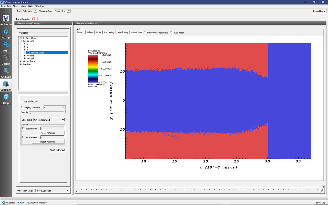
Fig. 485 The ionized charge states of argon during laser pulse propagation
Further Experiments
Try adding more charge states of Argon (past 6+) and find the limit of ionization that is achievable with this laser pulse.