Scattering off a Metal Sphere (metalSphere.sdf)
Keywords:
- Mie Scattering Off Metal Sphere
Problem description
The example describes the scattering of electromagnetic waves off a metal sphere. This phenomenon is often referred to as Mie scattering, where the radius of the sphere is comparable to the wavelength of the incident radiation.
An incident plane wave is launched toward the sphere. VSim computes the resulting fields in the vicinity of the sphere, within a computational domain by applying the proper boundary conditions around the surface of the sphere. The waves that exit the computational domain are absorbed into MAL layers.
The fields for points far away from the sphere, and beyond the computational domain are computed with the help of an analyzer that is part of the VSim distribution. The histories of the electric and magnetic fields are recorded along a closed surface known as a Kirchhoff box that lies within the MAL layers. This field information is then used to compute fields far away from the sphere center by applying the Kirchhoff integral theorem.
In this example, the radius of the metal sphere is set to equal 0.3367 times the wavelength of the incident radiation, which is 1m in length.
The wave is launched from the positive \(z\) direction, and the incident wave electric field is polarized along the \(x\) direction.
This example is set up as a cube, entirely parameterized off the NUM_WAVELENGTHS, WAVELENGTH and CELLS_PER_WAVELENGTH Constant. It is designed so that it may be easily adapted to take the radar cross section of any geometry, at any wavelength.
Two wavelengths on all sides are devoted to the MAL absorbing boundary conditions. The resolution of the grid corresponds to 16 cells per wavelength, near the middle of the typically used 10-20 cells. The time step (Parameter DT) is chosen to be very close to the Courant condition limit, calculated using the DX, CFL_NUM and DMFRAC Parameters.
The recording time for the Kirchhoff box is calculated using the parameters TBGNKBOX and TENDKBOX. TBGNKBOX is set by adding the turn on time of the excitation source, and 2* the time it would take to cross the diagonal of the RCS Box. TENDKBOX is set by taking TBGNKBOX, and then adding the amount of time to cross the entire RCS box, +2.5 periods. This allows for the collection of 2.5 periods of data.
The number of timesteps (Parameter NUM_STEPS) for the simulation corresponds to TENDKBOX/DT. Note that the number of steps in the simulation must be set by hand in Basic Settings, and verify that the value used in the Run Panel corresponds to this parameter.
This simulation can be performed with a VSimEM license.
Opening the Simulation
The Mie Scattering, Metal Sphere example is accessed from within VSimComposer by the following actions:
Select the New → From Example… menu item in the File menu.
In the resulting Examples window expand the VSim for Electromagnetics option.
Expand the Scattering option.
Select “Mie Scattering - Metal Sphere” and press the Choose button.
In the resulting dialog, create a New Folder if desired, and press the Save button to create a copy of this example.
All of the properties and values that create the
simulation are now available in the Setup Window as shown in
Fig. 316. You can expand the tree
elements and navigate through the various properties, making
any changes you desire. The right pane shows a 3D view of any
geometry, as well as the grid, if actively shown. To
show or hide the grid, expand the Grid element and select or
deselect the box next to Grid.
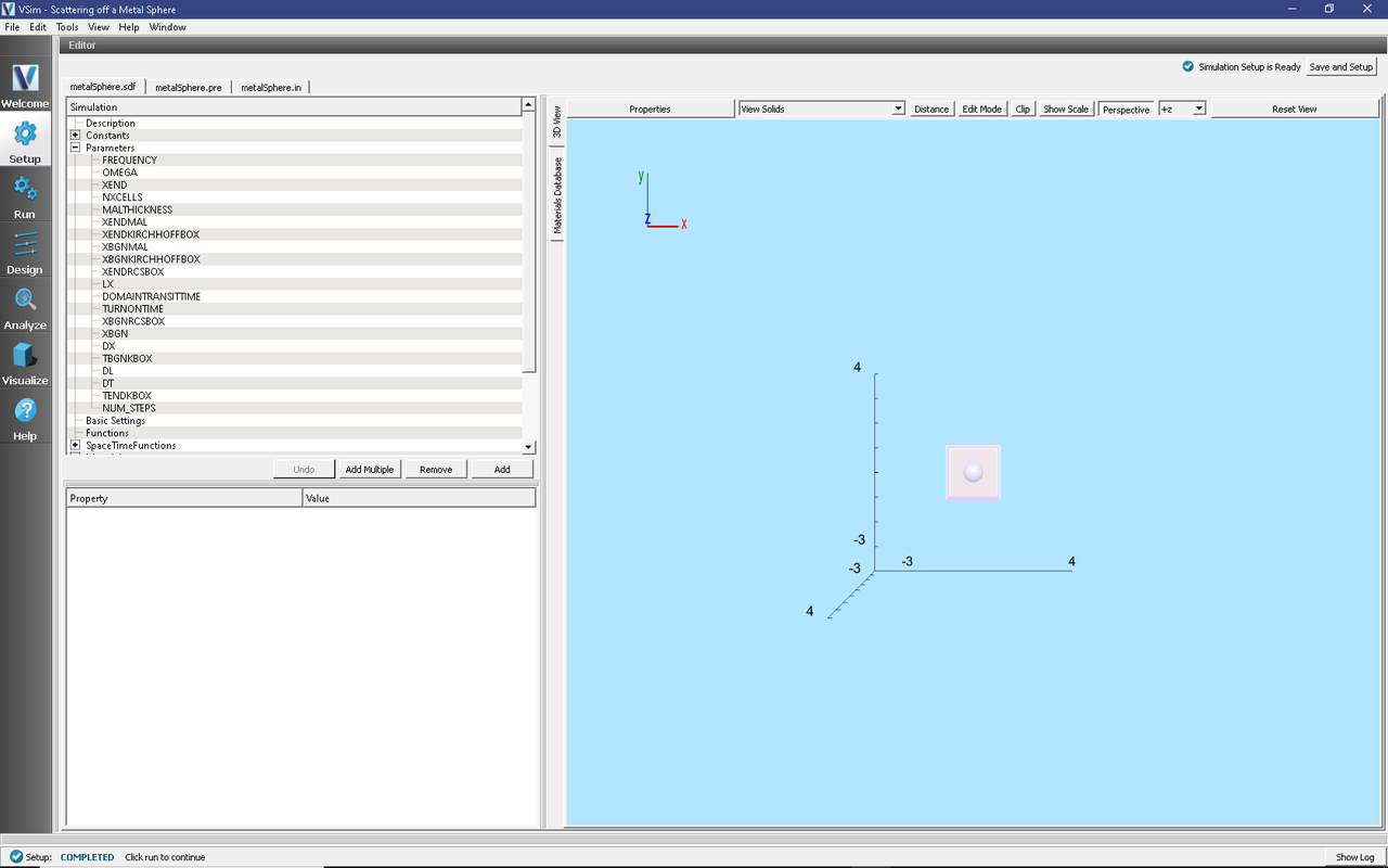
Fig. 316 Setup Window for the Mie Scattering example.
The Setup Window shows the Kirchhoff box, with the metal sphere at the center. To see the grid, click on the drop down menu of “Grids” on the left side panel. Check the box beside “Grid”. In order to view or change the wave frequency, click on the drop down menu “Parameters” and then click on “Frequency”. To view or change the direction of the incident wave or polarization, you can click on the drop down menu “Field Dynamics”, then the drop down menu “RCSBox”. Following this, check the box beside “rcsBox0”. The lower left panel displays a table with the wave property and its corresponding value.
Running the simulation
After performing the above actions, continue as follows:
Proceed to the Run Window by pressing the Run button in the left column of buttons.
To run the file, click on the Run button in the upper left corner of the window. You will see the output of the run in the right pane. The run has completed when you see the output, “Engine completed successfully.” See Fig. 317.
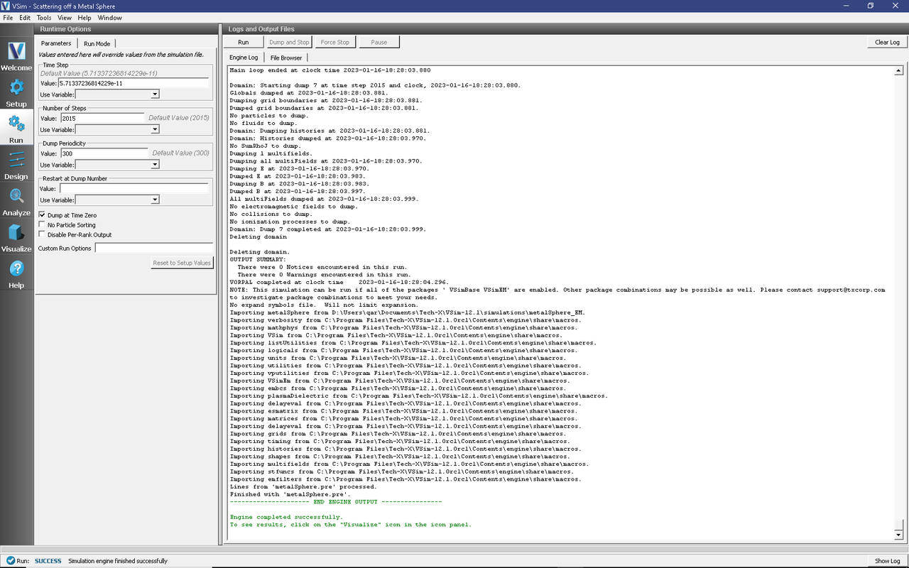
Fig. 317 The Run Window at the end of simulation.
Running in 3D, this simulation uses 2000 time steps. The run takes about 5 minutes on a 4-core 2.3 GHz processor.
Running the Analyzer
Proceed to the Analysis window by pressing the Analyze button in the left column of buttons.
Select the Default computeFarFieldFromKirchhoffBox.py Analyzer
Input values for the variables given on the left hand side of the screen. Check that these have the following values:
simulationName - metalSphere
fieldLabel - E
farFieldRadius - 1024.0
numPeriods - 0.25
numFarFieldTimes - 2
frequency - 0.3e9
numTheta - 45 (number of points in the theta direction)
numPhi - 90 (number of points in the phi direction)
zeroThetaDirection - (0,0,1)
zeroPhiDirection - (1,0,0)
incidentWaveAmplitude - 1.0
incidentWaveDirection - (0,0,1)
varyingMeshMaxRadius - 1.0
principalPlanesOnly - checked
Click the Analyze button near the top right of the window.
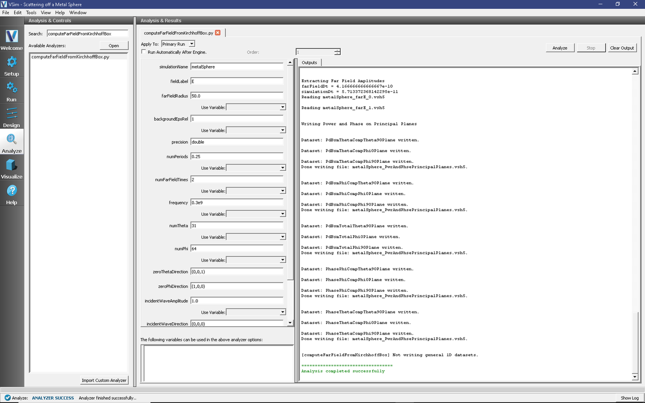
Fig. 318 The Analyze Window at the end of analyzer execution.
Visualizing the results
After performing the above actions, click on Visualize in the column of buttons at the left. The program will load the data and provide you with certain options.
One of the quantities that is of interest in such scattering phenomena is radar cross section (RCS) measured in dBsm. The RCS, sometimes designated as \(\sigma\), having units of \(m^2\), is given as
where \(R_s\) is the radial distance from scatterer, \(P_r\) is the power flux received at the point of interest, and \(P_i\) is the incident power flux. In MKS units the power flux is measured in \(W/m^2\). RCS in dBsm is given as
To obtain plots of this quantity, click on the drop down menu, Add a Data View. In this menu, choose 1-D Fields. There is a large list of options to choose from. Figure Fig. 319.
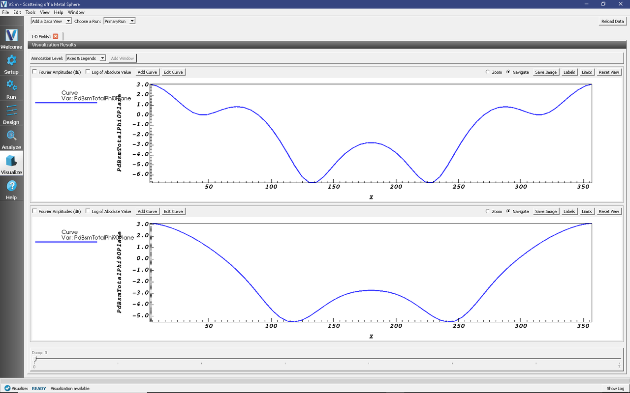
Fig. 319 The Visualize Window at the end of execution.
Further Experiments
You may try the example that includes a dielectric coating over the same metal sphere to compare the effects of such a coating over the RCS.